Sim-to-Real Transfer in Production Robotics: What Actually Survives Contact With Reality
Which sim-to-real transfer techniques actually survive production robotics? A practical guide to domain randomization, system identification, and the reality gap.
Simulation Is Cheap. Reality Is Not.
Every robotics team that has trained a policy in simulation has felt the same whiplash: a policy that clears 98% success in Isaac Sim or MuJoCo can fall into the low 60s on the factory floor. The exact drop varies by task, sensor suite, and cell — but the direction is consistent enough that experienced teams plan for it. Simulation gives you effectively infinite rollouts, clean labels, and free resets. Production gives you sensor drift, worn grippers, and a line that stops when the robot misses.
The gap is not academic. On a tightly takted line, a single missed pick can stall downstream stations and burn idle labor; the cost per minute depends entirely on your labor model and line design, but it is real and it compounds across a shift. A single missed pick at a 30-second takt can cascade into a two-minute stall once buffers drain, and at a loaded labor rate of $60–$120 per hour across the affected stations, that is $2–$4 of idle cost per incident — trivial once, ruinous at forty incidents a shift. And a policy that needs a skilled technician to reset it every forty cycles will never clear a return-on-investment review, no matter how good its simulated success rate looks. The teams that ship treat sim-to-real as an engineering discipline with measurable acceptance criteria, not a research milestone. (See our guide to production robot deployment checklists.)
Why Sim-to-Real Transfer Is the Hardest Problem in Robot Learning
The Promise vs. the Production Reality
Simulation's pitch is compelling: train millions of episodes overnight, iterate without touching hardware, and de-risk reinforcement learning before a single actuator moves. That promise is real — for exploration. But production imposes a different contract. A deployed policy must hold uptime and cycle-time guarantees, tolerate hardware wear, and pass a safety review that no simulator has ever signed off on. The gap between a research demo and a certified production cell is not a technicality; it is the whole job.
Consider the accounting. A simulation episode costs fractions of a cent; a real-world episode consumes hardware time, operator attention, and — if it fails badly — a broken end effector. A two-finger gripper replacement runs a few hundred dollars and a maintenance window; a crashed six-axis arm with a bent wrist can run five figures and a week of downtime. That asymmetry correctly pushes teams toward sim-heavy development, but it also breeds a dangerous optimism: because simulation is nearly free, teams over-index on simulated success metrics that have no production analogue. A policy that achieves 98% in sim has demonstrated that it can solve a mathematical problem. A policy that holds 99.5% first-pass yield across three shifts and two part variants has demonstrated that it can run a factory. The difference between those two numbers — roughly 1.5 points of failure — is where every hour of sim-to-real engineering gets spent. (Related: how to define robot acceptance criteria before deployment.)
Where the Reality Gap Comes From: Physics, Sensing, and Distribution Shift
The "reality gap" is the aggregate mismatch between simulated and real dynamics. It has four recurring sources:
- Unmodeled contact dynamics — friction, stiction, compliance, and deformation that physics engines approximate coarsely. MuJoCo uses a convex (soft) contact model, and Isaac Sim's PhysX uses a complementarity-based solver with configurable stiffness and iteration counts; both approximate contact stiffness and compliance rather than resolving true hard contact. The sub-millisecond stick-slip transitions that decide whether a peg seats or jams are exactly the events these models smooth over. A connector insertion that seats cleanly in sim at 0.1 mm clearance can jam on the real cell because the real peg chamfer deforms 20 microns under insertion force — a phenomenon no rigid-body solver represents.
- Sensor noise and latency — real cameras, force-torque sensors, and encoders add noise, dropout, and control-loop delay that simulators rarely model faithfully. A 30 ms camera-to-actuator latency, invisible in sim, can destabilize a closed-loop policy trained with instantaneous observation — this bites hardest on visual servoing and force-feedback tasks, where the feedback loop is tight. The fix is to model the delay (randomized delay augmentation, observation history stacks), not merely to acknowledge it. A common practical target: train with delay drawn uniformly from 0–50 ms so the policy degrades gracefully at the 30 ms you actually measure.
- Distribution shift — lighting, object pose, material finish, and part variability drift outside the training distribution. A matte anodized bracket and a polished stainless one look nothing alike to a vision model trained on the wrong finish. Add overhead LED flicker at 120 Hz, a pallet that arrives rotated 15 degrees off nominal, or a supplier switching from black to gray polymer, and a vision policy trained on a narrow capture set fails silently — confidently wrong rather than uncertain.
- Wear and calibration drift — grippers soften, belts stretch, and calibration decays over weeks. A policy tuned on day one sees a materially different robot by week six. A suction cup that held 5 N of vacuum on installation may hold 3 N after 40,000 cycles; a parallel jaw gripper's finger pads compress and its effective grasp width shifts by a millimeter.
Each source is individually manageable. The problem is that they compound, and a policy tuned to one gap often amplifies another. A policy made robust to lighting variance through aggressive augmentation may become slower to converge, which then interacts badly with latency it never saw in training. Robustness is not free — every axis of randomization you add trades some nominal performance for tail performance, and the art is knowing which tail you will actually hit.
What Actually Survives the Reality Gap
Domain Randomization — When It Helps and When It Hurts
Domain randomization (DR) varies simulation parameters — masses, friction, lighting, textures — so the policy learns to be robust across a distribution. It survives when randomization ranges match measured real-world variance. It fails in two predictable ways. Under-randomization produces a policy that has never seen the real variance and transfers poorly. Over-randomization produces a policy trained on implausible physics that converges slowly and becomes overly conservative — the classic "robust to everything, good at nothing" failure. The practical rule: calibrate randomization ranges against measured hardware data, not intuition. Teams that instrument their cells and set ranges from real telemetry consistently outperform teams that guess.
Concretely, for a 200 g to 900 g part family, set mass randomization to the supplier's stated part-to-part tolerance — often on the order of ±5–10% around measured values — not the ±50% that "feels safe." Friction coefficients should be drawn from a distribution fit to tribometer readings on the actual contact materials, and visual randomization should be anchored to a reference set of real captures. When ranges are set this way, DR is one of the highest-leverage techniques available; when they are set by folklore, it quietly manufactures the conservatism that kills cycle time. A team that randomizes friction from 0.1 to 1.5 "to be safe" trains a policy that grasps every object with a death grip and adds 200 ms per pick — which, at a 3-second takt, is a 7% throughput loss that shows up nowhere in the success metric. (See domain randomization calibration in practice.)
System Identification and Calibrated Physics
For manipulation, measuring beats guessing. System identification (sysID) fits simulation parameters — friction coefficients, link masses, joint compliance, actuator gains — to real trajectories. A calibrated simulator with narrower randomization often transfers better than a heavily randomized uncalibrated one, because the policy is trained on physics that resembles the cell it will run in. SysID is unglamorous and requires real hardware time, which is exactly why it gets skipped — and exactly why teams that do it gain an edge.
The practical workflow: excite the real robot with a set of identification trajectories, log joint states and torques, and fit parameters by minimizing trajectory prediction error, then validate the fit on held-out trajectories before trusting it. Calibration is not a one-time event. Because wear and drift are real, schedule periodic re-identification and feed the residuals into your randomization ranges. A useful discipline: hold out 20% of identification trajectories and require the fitted model to predict them within a stated error bound (for example, under 2 mm end-effector position error over a 2-second horizon) before the parameters are admitted into training. If the fit does not generalize to held-out data, it has memorized noise, not physics.
Learned Residual Dynamics and Online Adaptation
Even a well-calibrated simulator misses what it never modeled. Two techniques close the remaining gap without abandoning simulation:
- Residual dynamics models. Train a small learned model that predicts the difference between simulated and real next-state, layered on top of the physics engine. This keeps the simulator's structure while correcting its systematic errors. Because the residual is a correction rather than a full model, it needs far less real data than learning dynamics from scratch — often a few thousand real transitions suffice for a narrow task like a single insertion.
- Online adaptation. Use a short history of recent observations to infer the current regime (gripper wear, payload, surface finish) and adjust the policy or its inputs at runtime — the idea behind actuator-network-style adaptation, where a learned encoder maps recent state-action history to a latent context the policy conditions on. The encoder infers "this gripper is worn" or "this part is heavier" from the last few hundred milliseconds of behavior and conditions the policy accordingly, without ever being told the regime explicitly.
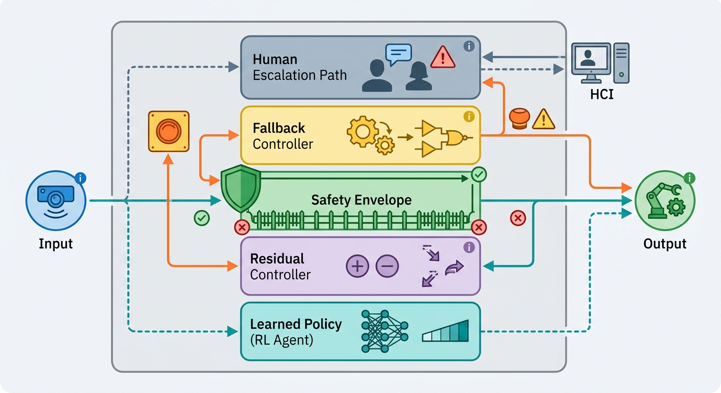
These are the techniques that let a policy survive week six, not just day one. They cost engineering effort, but they attack the compounding failure mode directly. The trade-off is real: residual models add inference latency and a second failure surface, and online adaptation can misdiagnose a regime and adapt in the wrong direction. Both need guardrails — bound the residual correction, and validate the adaptation encoder against held-out wear states before trusting it.
Measuring Transfer Instead of Claiming It
The most underrated sim-to-real technique is a disciplined evaluation protocol. Before a policy touches the production cell, define and measure:
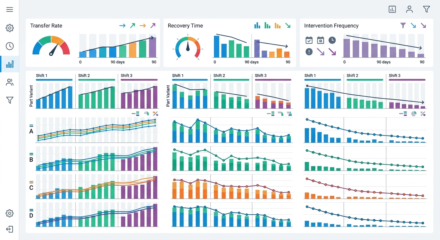
- Held-out real-world trials on the actual hardware, across the full range of part variants and lighting conditions the cell will see. A minimum of a few hundred trials per condition gives you a confidence interval tight enough to make a go/no-go call; twenty trials does not.
- Stress tests at the edges — worn gripper, degraded calibration, worst-case finish — not just nominal conditions. Deliberately install a gripper at end-of-life and confirm the policy still recovers.
- Recovery behavior — what the policy does after a near-miss, and whether it self-recovers or requires an operator. Measure the recovery rate and the recovery time separately; a policy that recovers 90% of the time but takes 30 seconds each time may still fail takt.
- Cycle-time distribution, not just mean, because the tail is what breaks takt. Report the 95th and 99th percentile cycle times alongside the mean.
A policy that passes nominal trials but has never been evaluated at the edges has not demonstrated transfer. It has demonstrated a best case.
Closing the Loop: Acceptance Criteria and Safety
Sim-to-real transfer is not done when the policy transfers; it is done when the cell passes acceptance. Tie every technique above to a measurable gate: fi