Real-Time Feature Stores: Architecture Patterns for Low-Latency ML Systems in 2026
Meta description: A real-time feature store prevents training-serving skew and enables low-latency ML inference. Learn the three serving patterns, online/offline store design, and how to avoid five common failure modes.
In 2025, a fraud detection team at a mid-size payments company spent three months building a state-of-the-art gradient boosting model. It achieved 0.94 AUC in backtesting. In production, it performed at 0.71. The problem wasn't the model — it was training-serving skew. The features used to train the model were computed differently than the features served at inference time. The model had learned patterns from clean, batch-computed historical data that didn't exist in the real-time serving environment.
Feature stores exist to solve exactly this problem. In 2026, they're no longer optional infrastructure for serious production ML — they're the architectural backbone that makes the gap between backtesting and production performance close to zero.
This article covers the architectural foundations of real-time feature stores: the dual-store design, three concrete serving patterns ranked by latency, and the failure modes that kill ML systems in production.
Why Feature Stores Are the Backbone of Real-Time ML
The standard ML workflow has a structural flaw baked into it. You train a model on historical data, then serve predictions on new data. If the features you compute for training don't match the features you compute at serving time — in definition, timing, or computation method — your model performs worse than your evaluation suggested.
This gap has a name: training-serving skew. It manifests in three common forms.
Definition skew occurs when training features and serving features are computed using different logic. A training pipeline might encode a categorical as an integer ID from a lookup table; the serving API might resolve that ID differently, or not at all. The model learns relationships based on ID mappings that don't exist at inference time.
Temporal skew occurs when training features use data from a time window that isn't available at serving time. Your training dataset uses a 7-day rolling average computed at batch time. At inference, you compute it from whatever data is currently available — which might be 30 seconds of data, producing a wildly different value.
Distribution skew occurs when the serving environment's data distribution differs from the training environment's, sometimes gradually (feature drift) and sometimes abruptly (concept drift). Without monitoring built into the feature pipeline, this skew is invisible until it causes a production incident.
A real-time feature store is the architectural layer that prevents skew by enforcing a single source of truth for feature definitions, computation logic, and serving paths. Feature store—prevents—training-serving skew. For low-latency ML systems — where inference latency is measured in milliseconds — this consistency requirement is especially acute, because you can't fall back on batch recomputation.
The Two Faces of a Feature Store — Online and Offline
Every production feature store has two interacting components: an offline feature store and an online feature store. Understanding what each does — and why both exist — is foundational to architectural decisions downstream.
The offline feature store holds historical feature values used to generate training datasets. Data typically lives in a data lake or data warehouse: S3, GCS, BigQuery, Snowflake, or Apache Iceberg-backed storage. Features are computed in batch, often using Spark or dbt, and stored as time-partitioned tables. When you generate a training dataset, you join feature snapshots at specific timestamps with your training labels. The offline store optimizes for storage efficiency and historical correctness, not for query latency. Offline feature store—generates—training datasets.
The online feature store holds precomputed feature values optimized for low-latency feature serving at inference time. Data typically lives in Redis, DynamoDB, or Cassandra. Queries return in single-digit milliseconds. The online store stores only the most recent (or most relevant) feature values per entity — user 12345's features as of the last materialization run. It doesn't store historical feature snapshots. Online feature store—serves—low-latency feature lookups.
The feature materialization pipeline is the bridge between offline and online stores. It runs on a schedule (hourly, minutely, or continuously) and copies feature values from the offline store to the online store. Feature materialization—transfers—features from batch to serving. The key architectural question: when does the materialization run, and how fresh do your features need to be?
Streaming features use change data capture (CDC) or stream processing to continuously update the online store as new events arrive. Features are fresher — potentially seconds-old — but the pipeline is more complex to operate.
The tradeoff is straightforward: tolerance for feature staleness versus operational complexity. For most recommendation and personalization use cases, 5–15 minute batch materialization is sufficient. For fraud detection and real-time risk scoring, sub-minute or streaming materialization is a hard requirement.
Architecture Patterns for Low-Latency Feature Serving
Three architectural patterns cover the majority of real-time feature store deployments. Choosing the right one is a function of your latency budget and the freshness requirements of your features.
Pattern 1: Precomputed Features with TTL Cache
The simplest pattern: compute features in batch, store them in the online feature store with a time-to-live, and serve directly.
Architecture flow: Event sources → Batch pipeline (Spark/dbt) → Online store (Redis/DynamoDB) → Feature API → Model inference.
Latency: < 10ms for feature retrieval, assuming the online store is in-region and the feature is a simple key lookup.
Best for: Features with moderate staleness tolerance (minutes to hours), high-cardinality entity features (user profiles, product catalogs), and lookup-heavy inference patterns.
How it works: The batch pipeline materializes features on a schedule. Each entity (user, product, device) has a feature record in the online store. At inference time, the model server calls the feature API with an entity key and receives the precomputed feature vector. No computation happens at request time.
Set a TTL that reflects your materialization cadence and staleness tolerance. If features are materialized hourly and you can tolerate 90-minute-old data, set a TTL of 5400 seconds with an on-hit refresh. This prevents serving stale features while materialization is delayed.
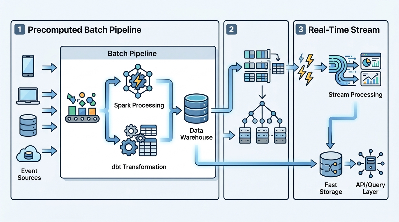
Pattern 2: Streaming Joins with Apache Flink or Kafka Streams
For features that require sub-minute freshness — rolling counts, windowed aggregations, real-time behavioral signals — precomputation on a batch schedule is insufficient. You need features to update as events happen.
Architecture flow: Event stream (Kafka/Kinesis) → Stream processing engine (Apache Flink/Kafka Streams) → Online store → Feature API → Model inference.
Latency: 20–50ms end-to-end for most streaming join patterns, dominated by stream processing window evaluation. Once a value is written to Redis, lookup adds only 0.5–2ms.
Best for: Real-time behavioral features (last-hour transaction count, rolling click-through rate, session duration), fraud signals, and any feature where minutes-old data is too stale. Streaming join—computes—real-time feature values.
How it works: As events arrive in the stream, the processing engine updates running aggregations — incrementing counters, updating rolling averages, recomputing windowed sums. The updated value is written to the online store immediately. The model serving layer sees feature values that reflect the state of the world within the last few seconds.
The hardest part of this pattern isn't the stream processing — it's joining streaming data with dimensional reference data (user attributes, product metadata) that changes less frequently. A user updates their profile in your CRM; that change needs to propagate into your streaming features within seconds. This typically requires a CDC pipeline feeding dimension changes into a second stream, which the stream processor joins against the fact stream.
Pattern 3: Hybrid Lookup with Real-Time Overlay
Most real-world systems use a mix of precomputed and streaming features. The hybrid pattern explicitly architectures for this.
Architecture flow: Event sources → Batch pipeline → Online store (base features) AND Event stream → Streaming pipeline → Online store (real-time overlay) → Feature API (merges both) → Model inference.
Latency: 50–200ms, depending on whether real-time computation is required at serving time.
Best for: Systems with heterogeneous feature freshness requirements — some features need to be real-time (fraud signals), others can be precomputed (user demographics, product categories).
The feature API fetches base features from the precomputed store and real-time features from the streaming store, then merges them into a single feature vector. The critical constraint: the merge must happen using the same logic in both training and serving, or you recreate the skew you were trying to eliminate.
Feature Engineering for the Prediction Moment
The single most important constraint in real-time feature serving is one that most feature store tutorials skip: every feature served at inference time must be computable from data available at that moment.
This is the prediction moment constraint. Prediction moment—constrains—feature availability. At the moment you make a prediction for user 12345, the feature "number of purchases in the last 7 days" can only use purchase events that have been recorded in your system. If the purchase event arrives in your data warehouse 5 minutes after the transaction due to processing lag, and you're serving predictions in real time, you cannot use the 7-day purchase count — it's not available yet.
This sounds obvious. In practice, it causes subtle leakage patterns that are difficult to detect.
Point-in-time correctness is the discipline of ensuring that when you generate a training dataset, you use feature values that would have been available at the moment the prediction was made. Point-in-time correctness—prevents—data leakage. This means joining features at specific timestamps — the feature value as of time T, not the feature value as of the training dataset creation time. Feast's get_historical_features API supports time travel queries; Hopsworks' getTrainingData also implements point-in-time joins. Both require proper configuration to enforce — default settings may not apply point-in-time semantics automatically.
The practical implication: your batch and streaming pipelines must track not just the feature value, but the feature timestamp — the time at which the feature value became available. Feature freshness—determines—prediction accuracy. Without this, there's no way to construct a training dataset that respects the prediction moment constraint, and your model will be trained on information from the future relative to the prediction moment.
The Leading Feature Store Platforms in 2026
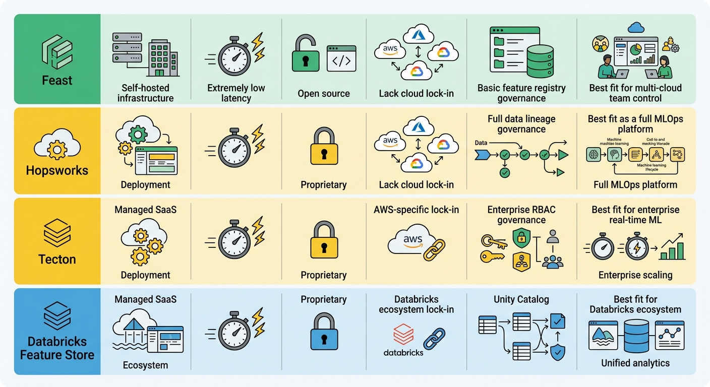
Feast remains the most widely deployed open-source feature store. Cloud-agnostic, mature Python SDK, deploys on GCP, AWS, and Azure. Offline store backed by BigQuery, Redshift, Snowflake, or Spark-compatible storage. Online store backed by Redis, DynamoDB, or SQLite. Feature materialization supports both batch and streaming modes. Best for teams that want infrastructure control and multi-cloud portability.
Hopsworks positions itself as a full MLOps platform with a feature store at its center. Strong integration with ML pipeline orchestration, model serving, and monitoring. Has native Milvus integration for embedding features. Offered as a managed service, reducing operational burden. Best for teams that want a unified MLOps platform with feature governance built in.
Tecton is a managed feature store built for enterprise low-latency ML. Primary design goal is sub-10ms feature retrieval at scale. Native support for streaming feature materialization (integrating with Kafka and Apache Flink), automatic feature computation from raw event streams, and built-in monitoring for feature drift and serving latency. Best for large-scale real-time systems requiring operational excellence at low latency. Requires AWS.
Databricks Feature Store is the choice for teams already invested in the Databricks Lakehouse. Integrates with Unity Catalog for governance and lineage tracking, and shares feature definitions between notebook exploration and production serving. Offline store backed by Delta Lake; online store defaults to DynamoDB on AWS and Azure Cosmos DB on Azure. Best for teams in the Databricks ecosystem.
Avoiding the Five Most Common Feature Store Failure Modes
1. Training-serving skew from non-deterministic feature transforms. If your feature computation uses non-deterministic operations — random sampling, unseeded hash functions, external API calls with variable responses — the features used in training will differ from those served in production. Fix: enforce deterministic feature definitions as a code review requirement. All feature computation code must be reproducible given the same inputs.
2. Stale features from infrequent materialization. If your materialization job runs hourly but your model uses features that decay in signal within 20 minutes, you're serving degraded predictions for 40 minutes per hour. Fix: profile your features' signal decay rate and set materialization cadence accordingly. Automate alerting when materialization is delayed.
3. Feature explosion without governance. As more teams use the feature store, the number of features grows without organization. Duplicate features with slightly different definitions proliferate. Feature registry—documents—feature definitions across teams. Fix: require feature registry entry with documentation, owner, and source lineage for every feature. Treat the registry as a first-class artifact with review and approval workflows.
4. Online/offline inconsistency. The offline store and online store return different values for the same entity and feature — because the computation paths diverged over time. Fix: the online store should be a materialized view of the offline store, using the same computation logic. Any change to feature computation must update both paths simultaneously or be gated behind a feature version bump.
5. Silent feature drift. Feature distributions shift gradually without triggering errors. Model performance degrades slowly, making the cause difficult to diagnose. Feature drift—degrades—model performance. Fix: implement Population Stability Index (PSI) monitoring for each feature. Alert when PSI exceeds 0.2 — a common industry threshold indicating significant distribution shift. Note that stable features (e.g., user birthdate) warrant tighter thresholds than volatile ones (e.g., real-time click counts). Track feature distribution histograms over time and surface them in the monitoring dashboard.
Implementing a Real-Time Feature Store — A Practical Checklist
Step 1: Define your latency budget. Model inference takes Xms. Feature retrieval must fit within your total serving budget. This determines which architecture pattern you can use. If you need p99 < 100ms end-to-end and your model takes 80ms, you have 20ms for features — forcing Pattern 1 (precomputed) with a fast online store.
Step 2: Audit upstream sources. Map every feature to its source system and the lag between event occurrence and data availability in that system. A feature is only as real-time as its slowest upstream dependency.
Step 3: Define the feature computation graph. For each feature, document: source system, computation logic, materialization cadence, TTL, and the timestamp field used for point-in-time correctness. This graph becomes your feature registry schema.
Step 4: Choose materialization cadence per feature group. Features with the same freshness tolerance should share a materialization pipeline. Group features by update frequency rather than materializing everything on a single schedule.
Step 5: Implement the feature registry. Document every feature: name, owner, description, computation logic (code reference), source systems, and entity keys. The registry is the contract between the data engineering team that builds features and the ML team that consumes them.
Step 6: Build monitoring before you launch. Population Stability Index monitoring for feature drift, SLO tracking for feature retrieval latency, data quality checks on upstream sources. Monitor the online store's hit rate — if feature lookups are failing frequently, your model's production performance will be worse than your evaluations suggest.
Conclusion
Real-time feature stores are the connective tissue of production ML systems. They prevent the training-serving skew that makes backtesting performance unreliable, enable low-latency feature serving at inference time, and provide the governance infrastructure for feature reuse across teams.
The three architecture patterns — precomputed features with TTL, streaming joins, and hybrid serving — cover the vast majority of production use cases. Choose based on your latency budget and feature freshness requirements, not on what's trendy. Most teams start with Pattern 1 and migrate to streaming or hybrid patterns as their freshness requirements crystallize.
The prediction moment constraint is non-negotiable: every feature served at inference must be computable from available data at that moment. Get this right and your training datasets will be honest representations of the world your model operates in. Get it wrong and you'll spend months debugging a model that worked in backtesting and disappoints in production.
Start with the implementation checklist. Audit your upstream sources, define your feature computation graph, and register every feature. The operational discipline of a well-run feature store matters more than the specific platform you choose.
If you're building real-time ML systems and want to go deeper on feature store implementation, explore our guide to streaming feature engineering — it covers the technical details of Apache Flink pipelines that this article introduces.
Explore next:
- [Streaming Feature Engineering with Apache Flink: From Event Streams to Feature Values]
- [Feast vs. Hopsworks vs. Tecton: A 2026 Feature Store Comparison]
- [Training-Serving Skew: Diagnosing and Fixing the Most Common Production ML Failure Mode]