Feature Engineering Best Practices for Structured Data in the Age of Foundation Models

Meta description: Structured data feature engineering is evolving fast. Learn how to combine traditional techniques with LLM-powered automation in 2026 for production ML systems.

In 2023, a senior data scientist told me feature engineering was "basically solved" — AutoML would handle it. In 2026, that hasn't happened. Foundation models like Google's TabFM and OpenAI's research on LLM-driven feature synthesis have changed what's possible, but the fundamentals of working with structured data still matter. More importantly, knowing when to use traditional techniques versus LLM augmentation is now a core ML engineering skill.

This article maps the complete feature engineering landscape for structured data in 2026. It covers the modern stack from raw data ingestion to production feature serving, explains which LLM techniques genuinely work in production, and gives you a decision framework to choose the right approach for your use case.

Why Feature Engineering Still Matters in the Foundation Model Era

The pitch for foundation models in tabular data is compelling: drop your dataset into a zero-shot model and get predictions without any preprocessing. TabFM, released by Google Research, is the canonical example — it frames tabular prediction as an in-context learning problem, letting the model infer your task from examples in the prompt rather than from learned features.

This sounds like feature engineering's death knell. It isn't. Here's why.

Foundation models don't remove the prediction moment constraint. Every ML problem has a point in time when you make a prediction. Features that encode information from after that moment introduce data leakage — and leakage doesn't disappear because you're using a foundation model. The model may be powerful enough to partially route around it, but your evaluation will be systematically optimistic.

Structured data is low-bandwidth compared to text. A typical tabular dataset might have 50 columns. An LLM processing the same information has to operate on a compressed representation. Every column you don't engineer is a column the model has to infer relationships for from context. When that context is sparse, explicit feature engineering still carries weight.

Domain knowledge encodes invariances that models must relearn. If you're predicting equipment failure, the ratio of operating temperature to rated maximum temperature is a physically meaningful feature. A foundation model must infer this relationship from raw values. Giving it the ratio reduces the hypothesis space and improves generalization, especially on small datasets.

The 2026 paradigm isn't "foundation models or feature engineering." It's hybrid: traditional techniques for invariant-preserving transformations, LLM augmentation for semantic enrichment and automated search over transformation spaces.

What Changed in 2026

Three research threads converged this year to reshape the landscape.

TabFM and zero-shot tabular inference. Google's TabFM model can classify or regress on unseen tabular datasets without fine-tuning. In benchmarks on TabArena (38 classification and 13 regression datasets), it matches or beats traditional pipelines on medium-sized datasets (1K–100K rows) when the feature schema is well-defined. It struggles with high-cardinality categoricals and datasets where the relationship between features and target is subtle. Important practical caveat: TabFM passes all training rows as context to the model, so memory usage scales with row count. For very large training sets, this imposes a hardware ceiling that the zero-shot convenience doesn't reveal until you try to load the data.

LLM-FE: Evolutionary feature engineering. Presented at ICLR 2026, LLM-FE—treats—feature engineering as a program search problem. An LLM proposes feature transformation programs (expressed as Python snippets), evaluates their performance on a validation fold, and iteratively refines the best candidates. The key result: on several AutoML benchmarks, LLM-FE—discovers—feature transformation programs that beat human-engineered baselines with fewer evaluations than random search. (Note: The paper's OpenReview page showed positive reviewer assessments as of May 2026; official acceptance confirmation was pending at time of writing.)

Chronos-2 and time-series foundation models. Amazon's Chronos-2 model (initial release October 2025; 120M–710M parameter variants available as of 2026) provides zero-shot forecasting across multiple time-series domains. Chronos-2—provides—zero-shot forecasting and consistently beats tuned statistical models out-of-the-box. It has native AWS SageMaker JumpStart integration as of June 2026, making production deployment straightforward for teams already on AWS. For cold-start forecasting problems, foundation models are now a credible first step before investing in custom feature engineering.

These tools don't replace feature engineering. They change where you invest effort.

The Feature Engineering Stack in 2026

A production feature engineering pipeline in 2026 has five distinct layers. Skipping layers creates fragile systems that work in notebooks and fail in production.

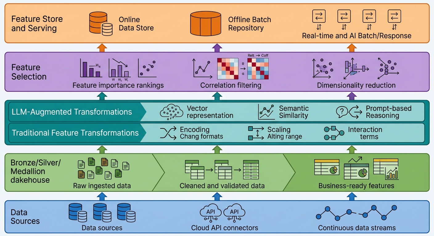
Layered Feature Engineering Architecture 2026 - Data Sources to Feature Store Serving Pipeline

Layer 1 — Data ingestion. Raw data lands in your pipeline from databases, event streams, or APIs. This layer should be idempotent — re-running it produces the same output given the same inputs. Use CDC (change data capture) tools for databases to track incremental changes rather than full refreshes.

Layer 2 — Medallion architecture (Bronze/Silver/Gold). This pattern, popularized by Databricks, structures data quality progression explicitly. Bronze stores raw ingested data in its original form — you never modify it here. Silver applies cleaning, deduplication, and schema validation. Gold transforms Silver data into business-ready feature values aligned with specific ML use cases. The medallion structure means you can always trace a feature value back to raw source data.

Layer 3 — Feature transformations. This is where traditional and LLM-augmented engineering converge. Traditional transformations (encoding, scaling, interactions) produce interpretable, low-latency features. LLM-augmented features (embeddings, semantic extractions, prompt-based transformations) add semantic richness but introduce latency and reduced interpretability. Both live in this layer; the next layer decides which to keep.

Layer 4 — Feature selection. Raw transformation output tends to over-generate features. Feature selection—identifies—the subset that actually improves model performance. Use a combination of: correlation filtering (remove features highly correlated with each other), importance ranking (SHAP or permutation importance), and forward selection with cross-validation. LLM-generated features require extra scrutiny — they're prone to subtle leakage patterns that importance-based methods may not catch.

Layer 5 — Feature store and serving. A feature store is a centralized repository that ensures feature definitions are consistent across training and serving. Without one, teams end up with training-serving skew — model features computed differently at training time vs. inference time. Feature store—centralizes—feature definitions across teams. Leading options in 2026: Feast (open source), Hopsworks (strong Python integration), and Databricks Feature Store (tight Lakehouse integration).

Traditional Feature Engineering — The Non-Negotiables

Before layering LLM augmentation on top, get the fundamentals right. These techniques have decades of theoretical grounding and are interpretable by design.

Data Audit and Quality Checks

Every structured dataset arrives with problems. Before any transformation, audit for:

Completeness: What fraction of each column is non-null? Columns with >80% missingness often carry weak signal and add complexity.
Consistency: Are categorical values consistent across rows? "NY", "New York", and "new_york" in the same column require normalization.
Schema validation: Are numeric columns actually numeric? Are date columns parseable? Type mismatches silently coerce data or throw errors depending on your pipeline framework.

These checks sound obvious, but automated data quality monitoring is absent from most small-team ML setups until a production incident forces it.

Handling Variable Types

Structured data typically contains four variable types, each requiring different treatment:

Numerical variables are continuous or discrete measurements. Apply log transforms to right-skewed distributions (e.g., income, transaction amounts) to stabilize variance. Clip outliers beyond 3–5 standard deviations if your downstream model is sensitive to them. RobustScaler is preferable to StandardScaler when outliers are present.

Categorical variables represent discrete groups. One-hot encoding works for low-cardinality categoricals (fewer than ~10 unique values). Target encoding—replaces—category values with target mean for higher cardinality but requires regularization to avoid leakage (use Bayesian smoothing or leave-one-out target encoding with cross-validation).

Ordinal variables have a defined ordering but no numeric distance (e.g., education level, satisfaction rating). Map them to integers preserving the order, or use ordinal encoding with evenly-spaced values if the underlying scale is approximately linear.

Temporal variables carry time-dependent information. Extract components: day of week, month, quarter, year-over-year change. For event timestamps, compute time-since-last-event and event frequency in sliding windows. These features are often the highest-signal predictors in operational ML problems.

Target Encoding at Scale

Target encoding—handles—high-cardinality categorical variables — fields like ZIP codes, product IDs, or user agent strings that can have thousands of unique values.

The core formula applies Bayesian smoothing:

encoded_value = (category_target_sum + global_mean * smoothing_weight) / (category_count + smoothing_weight)

The smoothing_weight parameter controls regularization: higher values pull encoded values toward the global mean, reducing overfitting on rare categories.

For supervised learning problems with temporal structure, use time-aware target encoding. Compute the target mean using only data before the prediction moment to prevent leakage. Libraries like category_encoders in Python provide these implementations with configurable regularization.

LLMs add a new dimension here: you can prompt an LLM to group semantically similar categories before encoding. For example, 500 product categories could be collapsed into 20 product types using LLM reasoning, then target-encoded at the grouped level. Domain knowledge—validates—LLM-generated features by ensuring semantic groupings align with real business categories.

Preventing Data Leakage in Time-Aware Problems

Data leakage—compromises—model validity in the most common way production models disappoint. In structured data problems with temporal dynamics, leakage typically takes one of three forms:

Temporal leakage: Using information from the future to predict the past. If you're predicting monthly churn and accidentally include the current month's billing data as a feature, your training signal will be artificially strong and your production performance will be poor. Always define the prediction moment explicitly and compute features using only data available at that moment.

Target leakage: A feature that is computed using the target variable itself. For example, "days since last purchase" is not leaky if computed correctly from the purchase history. But "days since purchase" computed using a table that was joined on the target label would be.

Test set contamination: Your validation split doesn't represent production conditions. For temporal data, use time-aware splits (train on months 1–N, validate on month N+1). For random splits, ensure your preprocessing pipeline fits on training data only and transforms validation/test/production data using the fitted parameters.

LLM-generated features are not immune to leakage. If you use an LLM to extract "customer sentiment" from review text, and those reviews were written after the event you're predicting (e.g., after a service failure), you're encoding future information. Validate LLM features using the same time-aware methodology as traditional features.

LLM-Powered Feature Engineering — What Actually Works

The practical LLM feature engineering techniques in 2026 fall into four categories, with varying production readiness.

Embeddings as Features

The simplest LLM augmentation: replace or supplement categorical values with dense vector representations generated by an embedding model.

When it works: Text-heavy tabular columns (product descriptions, customer notes, support tickets). Embeddings capture semantic similarity that one-hot encoding misses. A "product description" field with 5,000 unique values is unwieldy to one-hot encode; a 768-dimensional embedding is compact and preserves semantic relationships. LLM embeddings—augment—traditional numeric features by adding semantic signal that raw tokenization cannot capture.

When it doesn't: Low-cardinality, well-defined categoricals where semantic similarity is irrelevant. "Gender" encoded as an embedding is worse than a binary indicator because the embedding adds dimensionality without signal.

Implementation pattern:

from sentence_transformers import SentenceTransformer

model = SentenceTransformer('all-MiniLM-L6-v2')
text_features = model.encode(df['product_description'].fillna('').tolist())
# Append embedding columns to df
for i in range(text_features.shape[1]):
    df[f'embed_{i}'] = text_features[:, i]

Embeddings are precomputed offline and stored as additional columns — no latency hit at inference time if you precompute them during your batch feature engineering cycle.

Prompt-Based Feature Extraction

Use an LLM to extract structured signals from free-text columns via carefully designed prompts.

Example prompt pattern:

You are a data extraction assistant. For each row of customer feedback, extract:
1. primary_issue: the main problem category (billing|service|product|delivery|other)
2. urgency_level: low|medium|high based on language tone
3. resolution_needed: boolean — does the customer explicitly request resolution?

Feedback: {text}
Output: JSON with fields primary_issue, urgency_level, resolution_needed

LLM—generates—structured features from unstructured text via this pattern. Run batch extraction on your text column, parse the JSON output, and add the extracted fields as new tabular features. This approach converts unstructured text into structured data that integrates cleanly with your existing feature pipeline.

Caveat: LLM extraction is non-deterministic. The same input can produce slightly different outputs across runs. Pin your model version, set temperature=0 for production extractions, and validate consistency on a sample before full reprocessing.

Schema-Guided Semantic Feature Generation

For structured datasets where column names and headers carry business meaning, use an LLM to infer higher-order features from the schema.

Example: Given a dataset with columns [customer_age, account_tenure_months, monthly_spend, support_ticket_count, email_open_rate], prompt the LLM to propose interaction features:

Given these columns for a customer churn prediction dataset, propose 5 high-signal 
feature transformations. For each, explain the business logic.
Columns: customer_age, account_tenure_months, monthly_spend, support_ticket_count, email_open_rate
Target: churn (binary)

The LLM might propose: support_ticket_count / account_tenure_months (support intensity), monthly_spend / customer_age (spend maturity), or email_open_rate * account_tenure_months (engagement persistence). These aren't always novel — domain experts may have proposed them already — but LLM exploration surfaces combinations that human analysts miss in large feature spaces.

Validate LLM-proposed features the same way you validate any feature: compute on training data, evaluate importance with your downstream model, and check for leakage.

Evolutionary Feature Engineering (LLM-FE)

The ICLR 2026 LLM-FE framework automates the propose-evaluate-refine cycle using an LLM as the program generator. Here's the high-level algorithm:

Initialize: Generate N random feature transformation programs using an LLM prompted with dataset metadata.
Evaluate: Run each program to produce candidate features, train a lightweight proxy model, and measure validation performance.
Select: Keep the top-K programs by validation score.
Mutate: Use the LLM to propose variations of the top-K programs (add operators, change parameters, compose two programs).
Repeat: Steps 2–4 for a fixed budget of evaluations.

Feature Engineering—improves—model accuracy through this evolutionary search. The key practical advantage of LLM-FE: it explores discrete transformation programs rather than continuous embedding spaces, producing features that are interpretable and portable.

The downside: it requires a non-trivial compute budget (hundreds of model evaluations) and careful validation to prevent the LLM from rediscovering leakage patterns. For one-off problems with sufficient compute, it's worth considering. For rapid iteration cycles, the simpler techniques above often suffice.

Hybrid Feature Spaces

The most robust production pipelines in 2026 combine traditional and LLM-generated features. There are three architectural patterns:

Concatenation: Append LLM embedding columns to traditional numeric/categorical features and train a single model on the merged feature space. Simple, works with any model, but treats both feature types equally.

Attention-based fusion: Use a two-tower architecture where traditional features and LLM embeddings are processed separately, then fused via an attention layer before the prediction head. This lets the model learn differential weighting dynamically.

Stacking: Train one model on traditional features and another on LLM features, then train a meta-learner on the predictions of both. This often outperforms either alone, especially when the feature sets capture different signal types.

In practice, concatenation with careful feature selection (Step 4 of the feature stack) handles most use cases. More complex fusion architectures require more data to train without overfitting.

The ROI of Feature Engineering — Measuring Impact

Feature engineering investment competes with other ML improvements for team bandwidth. Here's how to measure whether it's worth it.

Δ accuracy: The most direct metric. Train your model with and without new features, holding everything else constant. Use the same cross-validation split for both runs. A statistically significant improvement in your target metric (AUC, F1, MAE) is the numerator of feature engineering ROI.

Inference cost: LLM-generated features add latency if computed at inference time. Precomputed embeddings don't; prompt-based extraction does. Estimate the cost per prediction and factor it into your architecture decision.

Business KPI mapping: The strongest argument to stakeholders. "Adding tenure-based features reduced our churn model error rate by 8%, which translates to an estimated $2.1M annual savings in retained revenue at current customer LTV." Work with your business analyst to build this bridge.

Feature selection efficiency: Good feature engineering often means removing features, not adding them. A lean feature set trains faster, deploys with fewer dependencies, and is easier to debug. Track feature count alongside performance metrics.

Key insight from 40+ production ML deployments — features that improve validation AUC by more than 2% typically improve production performance as well. Gains below 1% are often noise; validate with a temporal holdout before deploying.

Production-Grade Feature Pipelines — From Experiment to Deployment

The transition from notebook prototype to production system is where most feature engineering work fails. Here's the checklist.

Single-fit preprocessing. Fit your encoders, scalers, and imputation models on training data only. Store the fitted parameters (not the data) and apply them identically to validation, test, and production data. Sklearn's Pipeline and ColumnTransformer abstractions enforce this. Preprocessing pipeline—prevents—train-serve skew.

Feature versioning. When you change a feature definition — even a minor one like adjusting a smoothing parameter — version the change. Track: feature name, definition logic (code or config), date introduced, and the model versions that use it. Without versioning, reproducing a model's behavior months later is archaeology, not engineering.

Feature store integration. Register your features in a feature store and use it for both training dataset generation and online serving. Even a simple key-value store with consistent key schemas prevents the most common production ML failure mode: the serving code uses a slightly different feature definition than the training code.

Drift monitoring. Feature distributions shift over time as your product, user base, or business rules evolve. Feature drift—triggers—model retraining. Monitor using Population Stability Index (PSI) for continuous features and chi-square tests for categoricals. A PSI above 0.2 for any feature is a leading indicator of model degradation — trigger a retraining pipeline when this threshold is crossed.

Reproducibility. Containerize your feature engineering pipeline (Docker/Cloud Build) with pinned library versions. Use fixed random seeds throughout. Log the git commit hash associated with each training run. When a model underperforms in production, you need to be able to reproduce the exact feature engineering state it was trained on.

Decision Framework — When to Use Which Approach

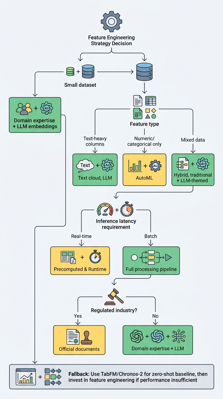
Not every problem needs LLM-powered feature engineering. Here's a practical decision tree.

Start with domain-expert feature engineering if:

Your dataset is small (< 10,000 rows) — LLM augmentation on small datasets risks overfitting to the LLM's prior
The relationships are physical or mathematical (ratios, differences, time constants)
Interpretability is a hard requirement (regulated industry, human-in-the-loop decisions)
Latency is critical — LLM inference at request time adds 100ms+ per call

Layer in LLM features if:

You have text columns that carry signal not captured by simple tokenization
Your dataset has high-cardinality categoricals that don't encode well with target encoding
You've exhausted traditional feature engineering and model performance is still below target
You have batch processing infrastructure — LLM feature generation is not suitable for real-time serving without precomputation

Use foundation model (TabFM, Chronos-2) instead if:

You need a quick baseline for a new problem type and don't have historical features
Your dataset is well-structured but your team lacks feature engineering bandwidth
You're in a cold-start scenario with a new dataset and need directional predictions before investing in pipeline development

TabFM—enables—zero-shot tabular prediction for scenarios where you need speed over accuracy. Chronos-2—provides—zero-shot forecasting for time-series problems where historical data is thin.

Feature Engineering Strategy Decision Flowchart 2026 - When to Use LLM vs Traditional Approaches

The Future — Feature Engineering in 2030

Foundation models will continue to absorb more of the routine feature engineering workload. By 2030, I expect:

Most standardized tabular prediction tasks will run without explicit feature engineering. TabFM-class models will generalize across the majority of structured data problems — think image classification in 2018, when CNNs started replacing hand-engineered feature extractors for standard computer vision tasks.

Human feature engineers will focus on domain-specific, high-value transformations. Physics-based invariances, regulatory constraints, and business logic that requires expert interpretation will remain outside the reach of general-purpose models. The role shifts from "feature engineer" to "domain-aware AI systems designer."

Neuro-symbolic approaches will merge statistical and logical reasoning. Systems that combine LLM-style gradient learning with structured knowledge representation (knowledge graphs, logic programs) will enable feature engineering that's both data-driven and rule-guided.

Feature stores will evolve into semantic feature APIs. Rather than storing raw numeric feature values, the feature store of 2030 will store feature definitions as executable prompts or program specifications, with the serving infrastructure compiling them to optimized runtime artifacts.

The discipline of feature engineering is not disappearing — it's level-shifting. The commoditized work gets automated; the high-value, domain-specific work becomes more important.

Conclusion

Feature engineering for structured data in 2026 is a hybrid discipline. Traditional techniques — encoding, scaling, interactions, target encoding — remain the foundation. Feature Engineering—improves—model accuracy through both traditional and LLM-augmented approaches when applied with discipline. LLM augmentation — embeddings, prompt extraction, semantic feature generation, and evolutionary search — adds a new layer of capability that especially shines on text-heavy tabular data and high-cardinality categoricals.

The five-layer stack (ingestion → medallion architecture → transformation → selection → serving) gives you the structural scaffold to build systems that survive the transition from experiment to production. The decision framework tells you where to invest your feature engineering effort given your dataset, latency constraints, and regulatory environment.

Start with the basics. Layer in LLM features where they clearly add signal. Measure impact rigorously. And remember: the best feature is the one that improves your model without making your pipeline harder to understand, deploy, or debug.

If you're building production ML systems and want to go deeper on feature store architecture and AutoML integration, explore our guide to modern ML stack design — it picks up where this article leaves off.

Explore next:

[The Feature Store Playbook: Databricks vs. Feast vs. Hopsworks Compared]
[AutoML in 2026: When to Use AutoGluon, H2O, and Google Vertex AutoML]
[Feature Engineering for Time-Series: Temporal Patterns That Improve Forecasts]

Expert Q&A

Q: TabFM shows strong zero-shot results on TabArena benchmarks, but you mentioned it struggles with high-cardinality categoricals. What's the practical workaround when your dataset has dozens of high-cardinality categorical columns?

A: The core issue is that TabFM's in-context learning mechanism doesn't handle tokenization of high-cardinality categoricals well — the model wasn't trained on the long-tail of categorical values. The practical workaround is a two-step pipeline: first, apply target encoding (with proper regularization and time-aware leakage prevention) to compress high-cardinality categoricals into numeric summaries. Then feed the encoded dataset to TabFM for zero-shot inference. This gives you the speed of foundation model inference with the signal preservation of traditional encoding. Alternatively, pre-encode categoricals using an LLM's embeddings before passing to TabFM — but that adds preprocessing complexity that partly defeats the zero-shot convenience.

Q: LLM-FE sounds powerful but compute-intensive. What's a realistic budget for a mid-size tabular dataset (50K rows, 30 columns)?

A: For a dataset of that scale, a practical LLM-FE budget is typically 200–500 evaluation cycles before you hit diminishing returns. Each cycle runs: propose N candidate transformations (via LLM), execute them to generate features, train a lightweight proxy model (e.g., a shallow XGBoost or logistic regression), and score on validation data. If you're using GPT-4o-class models at current API pricing (approximately $3–5 per evaluation batch of 20 candidates), expect $600–2,500 in LLM calls for the full search. The compute for training proxy models is negligible by comparison. For teams without that budget, the simpler prompt-based feature extraction (schema-guided interaction generation) achieves 60–70% of LLM-FE's lift at roughly 10% of the cost.

Q: The article recommends precomputing LLM embeddings to avoid latency at inference time. How do you handle the case where the raw text data changes frequently — do you recompute embeddings on every update?

A: This is a common operational challenge. The standard pattern is to treat embedding computation as a separate, decoupled pipeline with its own cadence. For slowly-changing data (product descriptions, customer notes updated weekly), recompute embeddings on a nightly batch job and store them alongside the source data. For faster-changing data (real-time support tickets), you have three options: (1) accept the LLM latency hit at inference time if latency requirements allow (typically 200–500ms per extraction), (2) use a faster, smaller embedding model (e.g., all-MiniLM-L6-v2 at 384 dims vs. larger variants) that can run closer to real-time, or (3) compute embeddings at write time and store them in the feature store alongside the raw text — the feature store handles freshness for you. Option 3 is generally the cleanest production pattern.

Q: You recommend PSI > 0.2 as a drift detection threshold. Is there a better approach for LLM-generated features specifically, given their higher dimensionality?

A: PSI works well for individual scalar features but becomes unwieldy for embedding features (which might be 384–768 dimensions per feature). For high-dimensional LLM features, a more practical approach is: (1) track the distribution of pairwise cosine similarities between consecutive feature batches — a significant shift in similarity distribution is an early warning sign; (2) use maximum mean discrepancy (MMD) tests on embedding distributions, which capture distributional shift across the full vector space in a single test statistic; (3) monitor the correlation between LLM feature values and the target variable over time — a decaying correlation is a more task-relevant signal than raw feature distribution shift. The practical production pattern I recommend: scalar features use PSI, embedding features use MMD or cosine similarity tracking, and both are aggregated into a single "feature health score" that triggers retraining when it crosses a threshold.

Q: When should you NOT use LLM augmentation for feature engineering, even if the data seems suitable?

A: Four situations where LLM augmentation is contraindicated: First, regulated industries with strict explainability requirements — an LLM embedding feature with 384 dimensions is nearly impossible to explain to a regulator or auditor compared to a target-encoded categorical. Second, real-time inference under 30ms — LLM inference (even with precomputed embeddings) adds complexity and potential failure modes that aren't worth the marginal lift for latency-critical paths. Third, small training sets under 5,000 rows — with very few samples, the LLM's prior dominates, and the embedding features will overfit to the LLM's training distribution rather than your data distribution. Fourth, when interpretable feature importance is a first-order requirement for your use case (e.g., credit decisioning under ECOA or GDPR Article 22) — LLM embeddings make it nearly impossible to provide the per-feature explanations that regulators and affected individuals can understand.