The Memory Bandwidth Wall: Why Inference Chips Are the Real 2026 Bottleneck
Inference is now the real AI bottleneck. Learn why memory bandwidth, not FLOPS, caps token throughput — and how the 2026 inference chip and HBM landscape is shifting.
The Memory Bandwidth Wall: Why Inference Is Now the Bottleneck
Training grabbed the headlines. Inference is grabbing the budget.
Through 2026, production AI spend has shifted decisively toward serving models rather than building them. Every chat completion, agent step, retrieval-augmented query, and code suggestion is an inference call, and the volume of those calls is compounding far faster than any training run cadence. Enterprises that once measured GPU demand in cluster-weeks now measure it in tokens per second per dollar, sustained around the clock.
That shift changes what "fast" means. The binding constraint for inference is no longer peak compute. It is memory bandwidth — the rate at which model weights and KV cache can be streamed into the arithmetic units that consume them. Chips marketed on teraflops can sit half-idle because memory cannot feed them fast enough.
This article covers the mechanics of why decode is bandwidth-bound, what the memory bandwidth wall means in practice, how the 2026 inference chip and HBM landscape looks, and what engineering and procurement leaders should do about it before the next refresh cycle locks in. (See also: GPU vs. inference accelerator: how to choose.)
The Bottleneck Moved — From FLOPS to Bytes
Training and inference reward different silicon. Training is a throughput problem that rewards peak matrix-multiply performance: large batches, long-running kernels, and enough parallelism to keep every tensor core busy. That is why training clusters are specified on dense FLOPS and interconnect bandwidth.
Inference is a latency-and-throughput problem that rewards memory movement. To generate a single token, an autoregressive model must read its weights — and the growing KV cache — from high-bandwidth memory into the compute units. The math is embarrassingly simple: if you can move N bytes per second and each token requires reading M bytes, your token rate is bounded by N/M regardless of how many FLOPS the chip can theoretically deliver.
A concrete example makes the ceiling tangible. A 70B-parameter model stored in FP8 occupies roughly 70 GB of weights. On a chip with about 3.35 TB/s of HBM3E bandwidth, a single decode step at batch size 1 must read those ~70 GB, capping throughput near 48 tokens per second per sequence — before any KV cache reads, and regardless of how many FLOPS the part advertises. Compute only re-enters the picture once batching raises arithmetic intensity.
Scale the example down and the wall follows you. A 7B-parameter model in FP16 occupies ~14 GB; on a chip with 1 TB/s of bandwidth, that caps a single stream near 71 tokens per second. A 405B-parameter model in FP8 needs ~405 GB of weights — well beyond the 141 GB of a single H200-class package — so it must be sharded across at least three chips, and every decode step pays a collective communication cost on top of the memory reads. The bandwidth wall does not disappear when you shard; it multiplies by the number of chips you had to add.
This is why a chip with modest peak compute but aggressive memory bandwidth can outperform a compute-heavy part on real serving workloads. For decode-heavy serving in 2026, bytes per second is the spec that sets the ceiling.
Why Decode Is Bandwidth-Bound
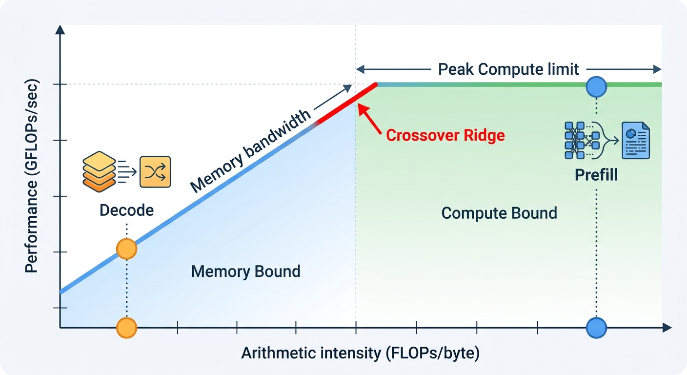
The roofline model makes this concrete. Arithmetic intensity — operations performed per byte moved — determines whether a workload is compute-bound or memory-bound. Prefill (processing the prompt) is compute-bound: large matrix multiplies reuse weights across many tokens. Decode (generating output one token at a time) is the opposite. Each new token requires a full pass over the model weights with almost no reuse, driving arithmetic intensity far below the roofline crossover point.
The KV cache sharpens the problem. Each decode step reads not only the weights but the accumulated key/value tensors for every token in context, for every concurrent sequence. Bytes moved per step scale roughly with (weights) + (KV cache size), and KV cache grows with batch size × sequence length. That is why long-context and agentic workloads — which re-read a growing conversation state — are so bandwidth-hungry.
Put numbers on it. For a 70B model with grouped-query attention, a KV cache entry costs roughly 320 KB per token at FP16 (80 layers × 8 KV heads × 128 head dimension × 2 tensors × 2 bytes). At a 32K-token context and a batch of 32 concurrent sequences, the KV cache alone is about 335 GB — larger than the weights, and read every step. At FP8 KV quantization that halves to ~168 GB, which is why KV quantization is one of the highest-leverage serving optimizations available.
The failure mode is predictable and common: a team provisions HBM for weights, deploys a long-context agent, and watches tail latency spike as the KV cache pushes the working set past capacity. The serving stack either evicts and recomputes (a latency cliff) or shards across chips (a bandwidth and interconnect tax). Neither shows up in a short-prompt benchmark.
Batching helps. Serving many requests concurrently amortizes weight reads across a larger effective batch and pushes arithmetic intensity back up. But batching has limits: larger batches grow the KV cache, consume more memory capacity, and add latency that hurts interactive workloads. You can batch your way toward compute-bound, but you pay in latency and memory capacity. Techniques such as PagedAttention (as implemented in vLLM), prefix caching, and KV quantization reduce the bytes moved per step, but they shift the wall rather than remove it. (Related: KV cache optimization techniques for LLM serving.)
What the Memory Bandwidth Wall Actually Means for Inference
Two memory properties matter, and buyers routinely conflate them.
- Capacity determines whether a model fits. A model whose weights and KV cache exceed HBM capacity must be sharded across chips or spilled to slower tiers, both of which add latency and complexity.
- Bandwidth determines how fast that model runs once it fits. This is the wall.
At small scale, capacity binds first — you cannot serve a model that does not fit. But once a model fits, bandwidth sets the ceiling on tokens per second, and adding more compute without more bandwidth yields diminishing returns. This is the practical trap: teams buy accelerators for peak TOPS, deploy a decode-heavy workload, and discover the chips are memory-starved. Utilization graphs show compute idle while HBM channels saturate.
KV cache compounds the pressure. As context windows grow and concurrency rises, the KV cache expands — consuming capacity and adding to the bytes that must be read and written each step. Long-context and agentic workloads, which re-read growing conversation state, are especially bandwidth-hungry. Context length and concurrency are bandwidth multipliers, not just capacity multipliers.
Decode does not care how many teraflops you bought. If your workload's arithmetic intensity sits below the roofline crossover, extra compute sits idle while HBM saturates. Bandwidth is what turns silicon into tokens — and prefill is where compute still earns its keep.
The 2026 Inference Chip and HBM Landscape
The market has responded. A distinct class of inference-optimized accelerators now competes alongside general-purpose GPUs, and — in our reading of public roadmaps and spec sheets as of early 2026 — the headline spec has migrated from peak dense FLOPS toward memory bandwidth per chip and bandwidth per dollar.
The vendor landscape spans several categories:
- General-purpose GPU platforms from established vendors, increasingly tuned for inference with larger HBM stacks and lower-precision formats.
- Inference-specialized accelerators from a growing field of startups and established silicon vendors, designed around memory movement and serving economics rather than training throughput.
- Hyperscaler custom silicon, built in-house to optimize cost per token for specific model families and serving stacks.
- Edge and mid-tier inference parts, where bandwidth-per-watt matters more than absolute throughput.
The common thread is HBM. HBM3E is in volume production with per-stack bandwidth in the roughly 1.2 TB/s range and 24–36 GB stacks; HBM4 is sampling with materially higher per-stack bandwidth and wider interfaces, and is expected to ramp through 2026–2027. Successive generations have raised both per-stack bandwidth and capacity, and the number of stacks per package has grown — but stacking more dies trades capacity against yield, power, and thermals. The practical result is a widening spread between chips on bandwidth-per-dollar and bandwidth-per-watt, which is now the axis that separates inference-optimized parts from repurposed training silicon.
The spread is wide enough to change buying decisions. A part with eight HBM3E stacks at 1.2 TB/s each delivers ~9.6 TB/s of aggregate bandwidth; a part with six stacks delivers ~7.2 TB/s — a 25% gap that shows up directly in tokens per second per dollar for decode-heavy traffic, even if the two parts advertise similar peak compute. Vendors that publish only dense FLOPS are telling you half the story; the stack count, stack generation, and power envelope tell you the rest.
There is a second-order trade-off worth naming. More stacks means more bandwidth, but also more package area, higher power draw, and tighter thermal budgets — which constrains how densely you can pack servers into a rack. A chip that wins on bandwidth-per-dollar can lose on bandwidth-per-watt if its power envelope forces you to halve rack density. That is why the evaluation discipline below asks for both ratios, not just one.
What Engineering and Procurement Leaders Should Do Now
The wall is real, but it is manageable with the right evaluation discipline.
- Benchmark decode, not just prefill. Prefill flatters compute-heavy parts. Measure time-to-first-token and steady-state tokens per second separately, at realistic batch sizes and context lengths. Use tools like vLLM's benchmark harness or GenAI-Perf to hold the serving stack constant across candidates so you are comparing silicon, not software.
- Specify bandwidth-per-dollar and bandwidth-per-watt. Ask vendors for HBM capacity, HBM bandwidth, and power at the SKU level, and compute the ratios yourself. These predict serving economics better than peak TOPS. A useful sanity check: divide your target model's weight footprint by the chip's bandwidth to get the theoretical single-stream token ceiling, then discount it 30–50% for KV reads and real-world efficiency.
- Model KV cache in your capacity plan. Size HBM for weights plus KV cache at your target concurrency and context length, not weights alone. Underprovisioning capacity forces sharding and erodes the bandwidth advantage. Build the calculation into your procurement spreadsheet before you shortlist parts.
- Test the workloads you actually run. Long-context, agentic, and multi-turn workloads are bandwidth-hungry in ways short-prompt benchmarks hide. Run your own traffic. A 512-token prompt benchmark will make almost any modern accelerator look adequate; a 32K-token agent trace will not.
- Account for total cost of ownership. Include memory tiering, interconnect, and the engineering cost of sharding when comparing chips — a cheaper part that forces complexity can lose on cost per token. Weight the engineering headcount of maintaining a multi-chip sharding pipeline as a real line item, not a footnote.
The next refresh cycle will lock in silicon for years. Buy bandwidth first, capacity second, and compute third — and validate all three against your real servi