The Inference Silicon Split: Why AI Budgets Are Moving from Training Clusters to Serving Fleets
Why AI infrastructure budgets are moving from training clusters to always-on inference serving fleets—and how cost-per-token and utilization reshape hardware ROI.
The Inference Silicon Split: Training vs. Inference Infrastructure
For most of the AI buildout, "GPU budget" meant one thing: capacity for training runs. That assumption is breaking down. Across hyperscaler capex commentary, neocloud procurement patterns, and rack-level designs, the money is increasingly tilting toward inference and serving—the always-on fleets that answer requests rather than the clusters that build models.
The thesis is simple and consequential: training and inference are no longer one workload with one hardware answer. Budgets are splitting along that fault line, and the split is reshaping how infrastructure buyers plan, procure, and model ROI. The directional case for an inflection around 2026 rests on three trends: AI moving from experiments to production, agentic workloads multiplying the number of calls per user, and serving demand becoming sustained rather than spiky. (Treat the timing as a thesis, not a forecast—operator guidance varies, but the direction of the mix shift is consistent.) When inference is always on, the hardware that serves it starts to look very different from the hardware that trains it.
The scale of the shift is worth putting numbers on. A single user prompt on a frontier model might consume a few thousand tokens; an agentic workflow that plans, calls tools, retrieves context, and self-corrects can consume tens of thousands of tokens per task and fan out into dozens of model calls. Multiply that across a production user base and the token volume behind "serving" dwarfs the compute footprint of the training run that produced the model. Training is a large, finite capital event; inference is a smaller, perpetual operating cost that compounds with adoption. That asymmetry—finite versus perpetual—is the root of the budget split.
The asymmetry shows up in the arithmetic. A frontier pretraining run might consume tens of thousands of GPU-months in a single multi-week burst and then be done. A production inference service serving, say, 10 million daily active users at 2,000 tokens per request generates on the order of 20 billion tokens per day—every day, for as long as the product lives. The training run is a one-time capital event measured in weeks; the serving load is an operating annuity measured in years, and it grows with every new user, feature, and agent loop. Vendors and operators have begun to reflect this in how they report: token throughput and cost-per-million-tokens are becoming the headline metrics of the serving era, the way FLOPs-per-dollar dominated the training era.
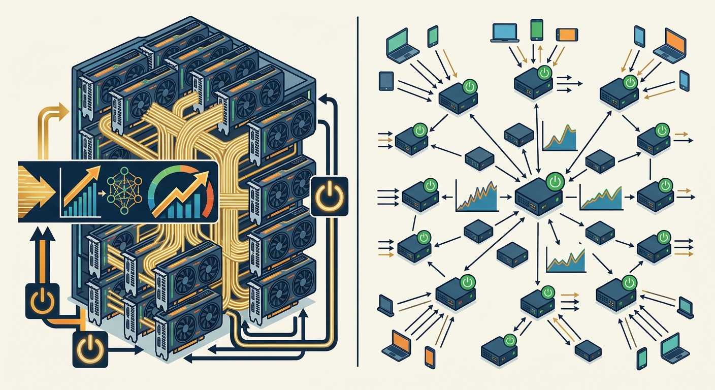
The Budget Line Is Moving Toward Inference
The clearest signal is in how capex is being described. Operators that once framed spend around "training capacity" now break out serving fleets, token throughput, and cost-per-request. Procurement mixes reflect it: a shift in the mix away from single-purpose training builds toward incremental serving capacity added in response to live demand. This is a rebalancing, not a retreat—frontier labs still commission very large training clusters—but the marginal dollar is increasingly a serving dollar.
This is best understood as a portfolio decision, not a single line item. A mature AI infrastructure plan now holds at least two distinct buckets with different lifecycles, utilization profiles, and failure modes. Treating them as one budget forces a compromise that optimizes neither. (See our breakdown of [how to size an inference fleet for peak concurrency].)
The portfolio framing has a practical consequence: the two buckets should be planned on different cadences and scored against different metrics. Training capacity is planned around model roadmaps and research milestones—lumpy, forecastable, and tolerant of slack. Serving capacity is planned around traffic growth curves, product launches, and SLA commitments—incremental, demand-driven, and unforgiving of slack. Mixing them in a single procurement motion tends to produce clusters that are overbuilt for serving and under-tuned for training, or the reverse.
What "Training Cluster" Capex Buys vs. What "Serving Fleet" Capex Buys
Training capex is front-loaded and bursty. You buy capacity for a finite run—a pretraining job, a fine-tune, a research sprint—and you want it available, tightly coupled, and fast for that window. Idle time between runs is expected and tolerated.
Serving capex is always-on and latency-bound. You buy capacity that must hold response times at the p95 while scaling with users, not with experiments. It grows in steps as demand grows, and every idle hour is a direct cost against live revenue. The purpose of the dollar is different, so the hardware answer diverges.
The lifecycle math makes the divergence concrete. A training cluster might run at high utilization for a six-to-twelve-week pretraining window, then sit largely idle for weeks while results are evaluated and the next run is scoped—an annualized utilization that can dip well below half. A serving fleet is provisioned for peak concurrency and paid for every hour of the year, so its economic viability depends on holding average utilization high enough to amortize fixed cost across tokens. As a rule of thumb, a serving fleet running at ~40% average utilization against peak-provisioned capacity is not "half idle"—it is likely structurally unprofitable, because depreciation and power bills arrive at 100% regardless. (The exact break-even depends on pricing, amortization period, and power contracts, but the direction is unforgiving.) That is why operators now treat utilization as a first-class operating metric rather than a capacity-planning afterthought. (Related: [why serving utilization beats raw FLOPS in production].)
A concrete comparison: a 1,000-GPU training cluster that runs at 90% utilization for twelve weeks and then idles for the rest of the year delivers roughly 20% annualized utilization, and that is acceptable because the run produced a model asset with multi-year value. A 1,000-GPU serving fleet provisioned for a Black Friday-style peak, running at 40% average utilization, is paying full depreciation and full power on 600 GPUs that generate no revenue. The training cluster's idle time is a scheduling inefficiency; the serving fleet's idle time is a cash-flow problem. Same hardware count, opposite economics.
Why Inference Economics Diverge from Training Economics
Training is a throughput problem. You want to maximize work per unit time across a long run, and you can tolerate batch latency—nobody sees the intermediate steps. That makes training sensitive to interconnect bandwidth and scale-out fabric performance, because the job is only as fast as the slowest link between accelerators. Data-parallel and tensor-parallel training spend much of their time synchronizing gradients and activations across the fabric, so a fabric bottleneck stalls every accelerator in the job simultaneously.
Inference is a latency and cost-per-token problem. Users see every millisecond. The workload is memory-bandwidth-sensitive: generating tokens means repeatedly reading model weights and KV-cache state, so the bottleneck is often how fast you can move data, not how many raw FLOPS you can throw at it. Utilization drives everything, because serving capacity is provisioned for peak and paid for around the clock.
The mechanics explain why. Autoregressive decoding generates one token at a time, and each token requires reading the model weights plus the growing key-value cache from memory. For a large model, the arithmetic intensity of a single decode step is low—you move far more bytes than you compute—so the workload is memory-bandwidth-bound rather than compute-bound. Training, by contrast, processes large batches across long sequences and can keep compute units saturated. This is why a chip with modest peak FLOPS but high memory bandwidth and a large, fast memory pool can beat a training-optimized part on tokens per second per dollar in production—and why serving silicon is increasingly designed around memory capacity and bandwidth per watt rather than raw matrix throughput.
The failure modes differ accordingly. A training job that hits a fabric bottleneck slows down uniformly—painful, but visible in the loss curve and fixable by rescheduling. A serving fleet that runs out of KV-cache headroom starts evicting or rejecting requests, which shows up as p99 latency spikes and 5xx errors under load—a customer-visible outage that no amount of extra FLOPS fixes. A serving fleet that is compute-rich but memory-poor will sit with idle tensor cores while the memory system chokes on decode. These are different failure signatures, and they demand different procurement bets.
Prefill vs. Decode: Two Bottlenecks Inside One Request
The single-workload framing hides a second split within inference. Every request has two phases with different hardware appetites:
- Prefill processes the full input prompt in parallel and is largely compute-bound—it behaves more like a short training step and benefits from raw FLOPS and high-bandwidth fabric.
- Decode generates output one token at a time and is memory-bandwidth-bound—it benefits from memory capacity and bandwidth (to hold weights and KV cache) more than peak FLOPS.
This is why serious serving fleets are tiered, not uniform: latency-critical interactive traffic, throughput-oriented offline batch, and long-context workloads get different silicon and different SLAs. It also explains techniques like disaggregated prefill/decode, where each phase runs on hardware tuned to its bottleneck. Buyers who spec a single "inference GPU" for all traffic leave money on the table in both directions.
The phase split also explains why long-context workloads are disproportionately expensive. A 100,000-token prompt makes prefill a substantial compute event—the model must process the entire context before emitting a single output token—and it inflates the KV cache that decode must carry, consuming memory that would otherwise serve concurrent requests. An operator mixing short chat traffic with long-document analysis on one uniform fleet will either over-provision for the chat case or under-serve the long-context case. Tiering by workload shape, and routing requests to the right tier, is now a core serving-design decision rather than an optimization.
Procurement Metrics That Actually Map to the Workload
Because the economics diverge, so should the scorecard. For serving, track:
- Tokens/sec per GPU at realistic batch sizes (not peak).
- $ per million tokens served, fully loaded with power and amortization.
- p95 time-to-first-token (TTFT) and p95 inter-token latency—the numbers users actually feel.
- Memory bandwidth and capacity per dollar, plus KV-cache headroom for long-context and concurrency.
- Sustained utilization against peak-provisioned capacity.
- Rack power and thermal density, since always-on fleets are power-bound, not just compute-bound.
Validate against standardized benchmarks (e.g., MLPerf Inference) and your own traffic replay rather than vendor peak numbers. The winning part is the one that holds latency at your p95 while driving cost-per-token down at your real concurrency—not the one with the highest spec-sheet FLOPS.
Two practical cautions. First, vendor peak numbers are almost always measured at batch sizes and sequence lengths that do not match production traffic; a part that leads on a headline benchmark can trail badly at your real concurrency and context mix. Second, benchmarks age: a part that wins on today's traffic replay may lose once your agentic workloads multiply call volume and stretch context windows. Build the replay harness, keep it current, and re-score the fleet every procurement cycle. The budget split is a durable structural shift—but which silicon wins inside each bucket is a moving target, and the operators who win are the ones who measure against their own workload rather than the spec sheet.