Mixture-of-Experts Routing in Production: Load Balancing, Expert Collapse, and Cost
Run mixture-of-experts models in production without surprises. Learn load balancing, expert collapse recovery, and MoE cost modeling for US AI teams.
Mixture-of-experts (MoE) architectures promise cheaper inference by activating only a fraction of parameters per token. The pitch is compelling: get dense-model quality at a fraction of the compute. But the moment you move an MoE model from a benchmark harness into live serving, routing behavior diverges sharply from training-time assumptions. Experts that looked evenly utilized in evaluation go hot under real traffic. Others go dark. And the cost savings you modeled quietly evaporate.
This article covers the three failure modes that dominate MoE production operations: load imbalance, expert collapse, and cost surprises. It's written for AI practitioners and engineering leaders who are either running MoE models today or evaluating them against a dense alternative. We'll move from why routing breaks, through the mechanics of inference-time gating, into telemetry, collapse recovery, and a cost model you can defend to finance. (For background on the architecture itself, see our overview of [sparse MoE model architecture].)
Why MoE Routing Breaks in Production (Not in Papers)
Training assumes a distribution. Production delivers a different one. The gating network was optimized against the token distribution in your training corpus, and live traffic rarely matches it. A customer support bot sees a different vocabulary mix on launch day than in the eval set. A code assistant absorbs a new language. A multi-tenant deployment blends dozens of workloads into a single routing stream.
Batching compounds the problem. Routing statistics are sensitive to batch composition, and production batches are heterogeneous by design—mixed sequence lengths, mixed tenants, mixed intent. A batch dominated by one workload can push a disproportionate share of tokens to the same experts. Sequence length variance does the same thing at a finer grain: long documents generate far more routing decisions per request than short queries, and those decisions cluster.
The Gap Between Benchmark Top-1 Accuracy and Serving Reality
Benchmark accuracy is a mean over a curated distribution. Latency is a tail metric driven by the worst-served requests. When a handful of experts absorb most of the traffic, the GPUs hosting them become the bottleneck while the rest idle. Your top-1 accuracy looks unchanged. Your p99 latency doubles. This is the central trap of MoE evaluation: aggregate quality metrics hide routing pathology because the pathology lives in the tail of the utilization distribution, not the mean of the accuracy distribution. (This is the same tail-versus-mean distinction that makes [LLM inference latency benchmarking] so easy to get wrong.)
How MoE Routing Actually Works at Inference Time
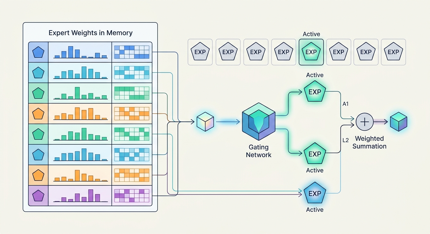
The mechanics are simple enough to state in one pass. A gating network—typically a small linear layer—scores every token against every expert. A top-k selection picks the k highest-scoring experts. Tokens are dispatched to those experts, processed, and recombined as a weighted sum using the gate scores as weights.
Two clarifications matter for operations. First, "sparse" refers to compute, not memory. Every expert's weights must be resident on the serving hardware regardless of whether a given token touches them. An 8×7B model holds roughly 56B of expert parameters in VRAM—plus attention blocks, embeddings, and the router, which are not multiplied by the expert count—while each token activates only a fraction of that expert capacity. Second, routing policy is model-specific. Top-1 versus top-2, shared-expert designs, and fine-grained expert partitioning all change what "balanced" means and how you should instrument it. There is no universal MoE routing dashboard—you build one per architecture.
Token-to-Expert Assignment and Top-k Gating
Top-1 routing sends each token to a single expert. It's the cheapest option and the most fragile: any imbalance directly translates to hot-spot contention. Top-2 routing doubles the compute per token but smooths the load and often improves quality. Shared experts—always-on experts that process every token—are designed to absorb common patterns, which in principle leaves the routed experts more room to specialize. When you tune anything downstream, remember that capacity factor, temperature, and top-k interact; changing one without re-measuring the others is how you get a regression you can't explain.
Capacity Factors and Token Dropping
The capacity factor (CF) sets a per-expert token budget. The precise formula is:
capacity per expert = CF × (tokens in batch) / (number of experts)
With CF = 1.25 and 8 experts, each expert can hold 1.25/8 of the batch's tokens—25% headroom above a perfectly uniform split. When an expert exceeds its budget, the excess tokens are dropped. What "dropped" means depends on your top-k setting and implementation: in top-1, a dropped token loses its only route and its output contribution vanishes; in top-k, it loses one of k contributions, and whether the remaining weights are renormalized varies by implementation. Check your serving stack's behavior rather than assuming.
Dropping is often silent. Many serving stacks expose drop counters (vLLM and SGLang, for example, surface routing and drop metrics), but if you're not watching them, the symptom appears as a quality regression, not an error. If your capacity factor is too tight, you'll see accuracy drift under skewed traffic; too loose, and you pay for padding and wasted memory. Capacity factor is a live tuning parameter, not a build-time constant—but changing it at runtime requires re-validating output quality, because the router was trained under a different effective capacity.
Load Balancing: From Auxiliary Loss to Production Telemetry
MoE models are trained with an auxiliary load-balancing loss that penalizes uneven routing. It works—during training, on the training distribution. It is not a production guarantee. The auxiliary loss is a soft constraint baked into weights, and weights don't adapt when traffic shifts.
That's why production load balancing is a telemetry problem first and a tuning problem second. (The instrumentation patterns overlap with our guide to [LLM observability and serving telemetry].)
Auxiliary Load-Balancing Loss and Its Limits
The auxiliary loss pushes the router toward uniform assignment by penalizing the deviation between each expert's token share and the uniform expectation. Two limits matter operationally. First, it is a soft penalty optimized jointly with the language-modeling objective; the model will trade some balance for quality, and that trade is invisible to you at serving time. Second, it is frozen once training ends. A model trained to balance on English support tickets carries no mechanism to rebalance when 40% of your traffic becomes Japanese. The loss shaped the weights; it does not watch the router.
This is also why bias-based, loss-free balancing (adding a per-expert routing bias that is updated from observed load rather than through the gradient) has gained traction in recent training recipes: it decouples balance from the quality objective. If you're training your own MoE, prefer it. If you're serving a pretrained one, you inherit whatever balance the original recipe produced—and must monitor it yourself.
Expert Collapse: What It Is and How to Detect It
Expert collapse is the end state of load imbalance: routing mass concentrates on a shrinking subset of experts, and the rest receive little or no traffic. In training it's a positive-feedback loop—an expert that wins early tokens gets more gradient, becomes better, and wins more. At inference, collapse persists as a structural property: the dark experts are still resident in VRAM, still consuming memory bandwidth and capacity, but contributing nothing. You are paying full memory cost for a fraction of the model.
Detect it with a per-expert token-share histogram over a rolling window, not a single batch. The signature is a long tail: a few experts above 2× uniform share, several below 0.1×. Track it per tenant and per workload class—collapse that's invisible in aggregate traffic often shows up cleanly when you segment by customer.
Recovery Levers
Once you've confirmed collapse, the levers, roughly in order of cost:
- Router temperature. Flattening the gate distribution (raising temperature) spreads tokens across more experts at some quality cost. Cheap to try, easy to overdo.
- Capacity and drop policy. Loosening CF or enabling shared-expert overflow reduces the hard cutoff that can starve experts under skewed batches.
- Routing bias adjustment. If the architecture supports per-expert bias terms, nudging them toward underused experts rebalances without retraining.
- Fine-tuning with a stronger aux-loss coefficient. The real fix if the collapse is severe; requires labeled data and a retraining cycle.
- Expert re-initialization. A last resort for training-time collapse; not applicable to a frozen served model.
None of these is free, and all of them must be validated against the tail latency and quality metrics from the previous section—not just aggregate accuracy.
The Cost Model You Can Defend to Finance
The savings claim for MoE is real but narrower than the pitch. Be precise about which cost you're reducing.
Memory is not saved. Total parameter count drives VRAM residency. An MoE with 56B expert parameters plus non-expert overhead needs hardware sized for the total, not the active fraction. If your dense baseline is a 13B model and your MoE is 8×7B, you are not saving memory—you are spending more of it.
Compute is saved, conditionally. Active parameters per token drive FLOPs. That is the genuine win, and it shows up as higher throughput per GPU when batches are large enough to keep the hardware busy. At small batch sizes, MoE inference is memory-bandwidth-bound—you stream expert weights for very few tokens—and the compute savings don't materialize. Model your cost at your actual batch sizes and sequence lengths, not at peak throughput.
Imbalance is a cost line. When a few experts saturate, the GPUs hosting them gate your p99 while the rest idle. Effective utilization drops below nameplate, and you provision for the hot expert, not the average. Budget for this explicitly: measure per-expert utilization and size capacity for the skew, or invest in balancing to recover the headroom.
Dropping is a quality cost. A tight capacity factor saves memory and compute and silently costs accuracy. Put a number on the accuracy you're willing to trade for the throughput gain, and monitor drop rates against it.
A defensible model has four terms: total-parameter memory cost, active-parameter compute cost at your real batch profile, imbalance-driven overprovisioning, and the quality cost of drops. The first is fixed and often higher than dense. The second is the savings. The third and fourth are the surprises—and they are the ones that make the spreadsheet and the invoice disagree.
Instrumentation Checklist
Before you trust any MoE cost or quality number, confirm you can measure:
- Per-expert token share, per tenant and per workload class, over a rolling window.
- Drop rate and the renormalization behavior of your serving stack.
- p50 and p99 latency segmented by which experts a request touched.
- Effective GPU utilization versus nameplate, per expert-hosting device.
- Active versus total parameter counts, stated separately in every capacity plan.
If you can't produce all five, you don't yet know whether your MoE is saving money or quietly losing it.