Mixture-of-Experts Routing in 2026: What Sparse Frontier Models Actually Cost You
How mixture-of-experts routing drives real inference cost in 2026—memory residency, interconnect tax, capacity factors, and what to ask before you deploy.
The Sparse Paradox: Fewer FLOPs, Bigger Bills
Sparse frontier models look like a bargain on paper. A 600-billion-parameter mixture-of-experts (MoE) model might activate only 40 billion parameters per token, so vendors quote per-token compute costs that appear to undercut dense models by a wide margin. Then the invoice arrives—or the p95 latency spikes—and the math stops working.
The gap between advertised and actual cost comes down to one thing: routing. Every token that enters an MoE model is assigned to a small subset of expert subnetworks, and those routing decisions determine your real inference cost, your latency profile, and how consistent the model's output quality is from request to request. You can't evaluate a sparse model by its parameter count any more than you can evaluate a car by its horsepower rating alone.
This article breaks down how MoE routing works in 2026's frontier architectures, where the hidden costs accumulate, and what to ask before you commit to a sparse model in production. If you're modeling TCO, writing serving infrastructure, or negotiating a vendor contract, the details below are the ones that move the number. (See also: How to Model LLM Inference TCO Before You Sign a Contract)
Why Every Frontier Lab Went Sparse
Dense transformer scaling hit a wall. To improve quality, you historically had to add parameters and spend more FLOPs on every token—training and inference costs scaled in lockstep with capability. MoE architectures broke that coupling. By routing each token through only a fraction of the network, labs decoupled total parameter count from per-token compute.
The result is a generation of frontier models with enormous total parameter counts and comparatively modest active parameter counts. Vendors lean hard on the big number in marketing, because total parameters correlate with knowledge capacity and benchmark scores. The smaller number—active parameters—is what drives per-token compute. But per-token compute is only half the bill. The other half is the fixed cost of keeping every expert resident in memory, and that scales with total parameters. Keep both numbers in view.
| Metric | What It Governs | Where You Feel It |
|---|---|---|
| Total parameters | Model capacity, knowledge storage, memory residency | GPU memory footprint, minimum GPU count, hardware floor cost |
| Active parameters | Per-token compute | Latency, throughput, variable compute cost |
That distinction is the single most important thing to internalize about sparse models. A model with 8x the total parameters but the same active parameters as a dense baseline does not cost 8x more per token to compute—but it can cost far more to host, because you must provision memory for all the weights. The sparsity ratio (total ÷ active) tells you how far those two cost curves diverge. That ratio varies widely across model families; treat any single figure as illustrative, not canonical. (Related: Dense vs. Sparse Model Hosting Costs Compared)
How MoE Routing Actually Works
At each MoE layer, a router (gating network) scores every token against every expert and dispatches it to the top-k highest-scoring experts—commonly k=2, though the exact value (and expert count) is model-specific. The token's output is a weighted combination of those experts' results. A few routing details have outsized downstream effects.
Token Choice vs. Expert Choice Routing
In token choice routing, each token picks its top-k experts. It's the dominant scheme because it's simple and preserves causality for autoregressive generation. The downside: tokens cluster onto popular experts, creating imbalance that must be corrected with auxiliary losses or, in fixed-shape serving, token dropping.
Expert choice routing flips the assignment—each expert selects its top-capacity tokens. This guarantees near-perfect load balance and often improves throughput, but it complicates autoregressive decoding and can let experts "hoard" tokens in ways that hurt quality. Most 2026 frontier serving stacks use token choice with careful balancing; expert choice shows up more in research and specialized batch workloads.
Load Balancing and Capacity Factors
To prevent a handful of experts from becoming bottlenecks, training adds an auxiliary load-balancing loss, and fixed-shape serving enforces a capacity factor—a per-expert token limit. When an expert overflows, excess tokens are either dropped or rerouted to a fallback path.
It's important to separate the two contexts. Token dropping is primarily a training-time and fixed-batch phenomenon. Modern serving stacks that use continuous (dynamic) batching typically size or disable the capacity factor so that no tokens are dropped, trading memory headroom for quality. If your vendor's server drops tokens at inference, that's a red flag worth asking about—it means quality degrades on skewed inputs, and the degradation is invisible in aggregate benchmarks.
A tight capacity factor improves throughput predictability but increases dropping; a loose one preserves quality but inflates memory and compute headroom. The capacity factor your vendor ships with is a cost-quality dial you usually can't see. (Deeper dive: Capacity Factors and Token Dropping Explained)
Routing is where a sparse model's advertised efficiency meets the realities of your workload. Two teams running the same model with different traffic patterns can see wildly different costs per token.
The Hidden Costs of Sparse Models
Inference Cost: You Pay for Memory, Not Just Compute
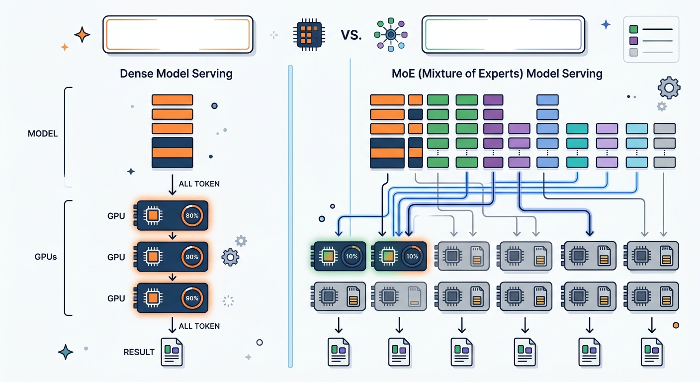
Here's the core economic fact of MoE serving: every expert must be resident in memory even though only a few activate per token. A model with 600B total parameters needs to fit—or be sharded across—enough GPU memory to hold all 600B worth of weights, regardless of how few FLOPs each token consumes.
This makes MoE inference memory-bound at low-to-moderate batch sizes, which is where most interactive and agentic workloads live. You're paying for HBM capacity and memory bandwidth, not arithmetic throughput. That's why cost-per-token benchmarks built on dense models mislead: they assume compute is the bottleneck, but for sparse models at interactive batch sizes the binding constraint is how many GPUs you need just to hold the weights, and how fast you can stream them.
The crossover matters for capacity planning. As batch size grows, you amortize weight streaming across more tokens, arithmetic intensity rises, and the workload becomes compute-bound—at which point active parameters take over as the cost driver. The practical implication: MoE is relatively more attractive for high-throughput batch workloads and relatively less attractive for latency-sensitive, low-batch traffic. Benchmark your actual batch profile, not a vendor's. (See: Why GPU Memory Bandwidth Drives Inference Cost)
Expert Parallelism and the Interconnect Tax
Because all experts must be resident, large MoE models are typically served with expert parallelism—experts distributed across multiple devices. At every MoE layer, tokens must be sent to whichever device holds their assigned experts and the results sent back. This is an all-to-all exchange, and it is the dominant hidden cost in MoE serving.
Two properties make it expensive. First, the volume is large: every token's activation vector traverses the network at every MoE layer, so total traffic scales with batch size × sequence length × hidden dimension × number of MoE layers. Second, the cost depends heavily on where the experts live. If all experts for a layer fit within a single NVLink-connected node, all-to-all is fast. If they spill across nodes onto InfiniBand or Ethernet, the same exchange becomes the latency bottleneck—and p95 latency, not average, is what your users and your SLOs feel.
This is why expert-parallel topology is a first-order procurement question. A model whose experts fit in one high-bandwidth node will behave very differently from the same model sharded across a multi-node cluster, even though the parameter count and FLOPs are identical. Vendors rarely advertise which regime they operate in. Ask.
The Costs That Don't Show Up in FLOP Math
Beyond memory residency and interconnect, several factors inflate real-world MoE cost:
- Minimum viable GPU count. You can't run the model on fewer GPUs than it takes to hold all weights, so you pay a fixed floor regardless of traffic. Idle capacity is expensive capacity.
- Quantization interacts with routing. Aggressively quantizing expert weights saves memory (directly reducing GPU count) but can perturb router scores and shift expert selection, with quality effects that differ by workload.
- Tail latency from routing skew. Workloads with skewed token distributions concentrate load on popular experts, and the slowest request in a batch sets your p95. Uniform-input benchmarks systematically understate this.
What to Ask Before You Commit
Before you sign, get answers to these:
- Sparsity ratio and top-k. What are total vs. active parameters, and what is k? This sets both your compute curve and your memory floor.
- Expert-parallel topology. Do all experts for a layer fit within one NVLink node, or does serving cross node boundaries? This determines whether all-to-all is cheap or dominant.
- Batch-size fit. At what batch size does the workload shift from memory-bound to compute-bound, and where does your traffic sit?
- Capacity factor and dropping. Does the serving stack drop tokens at inference, and under what input distribution?
- Quantization scheme. What precision are expert weights stored in, and has router stability been validated post-quantization?
- Telemetry. Does the vendor expose routing distribution, expert utilization, and all-to-all latency so you can diagnose regressions?
The models are genuinely more efficient than their dense predecessors on the right workload. The trap is assuming the advertised per-token number is the one you'll pay. It's the one that applies when memory, interconnect, and routing all cooperate—and your job is to verify that they will.