Diffusion Language Models vs Autoregressive: Where Each One Actually Wins
Compare diffusion language models vs autoregressive LLMs on quality, latency, throughput, and tooling — plus a decision framework for US AI teams.
Diffusion Language Models vs Autoregressive LLMs: Where Each One Actually Wins
Autoregressive (AR) LLMs run most production AI today. But diffusion language models have moved from research curiosity to a credible alternative in specific niches — and the architecture decision now has real budget and SLA consequences. This is not a winner-take-all comparison. Each architecture wins on different axes: latency profile, controllability, throughput, and output quality. What follows is a practitioner's decision framework for matching architecture to workload, not a hype cycle recap. If you're choosing AI infrastructure in 2026, the question isn't which model is "better" — it's which failure mode you can afford.
How Autoregressive and Diffusion Language Models Actually Differ
Autoregressive decoding: token-by-token, left-to-right
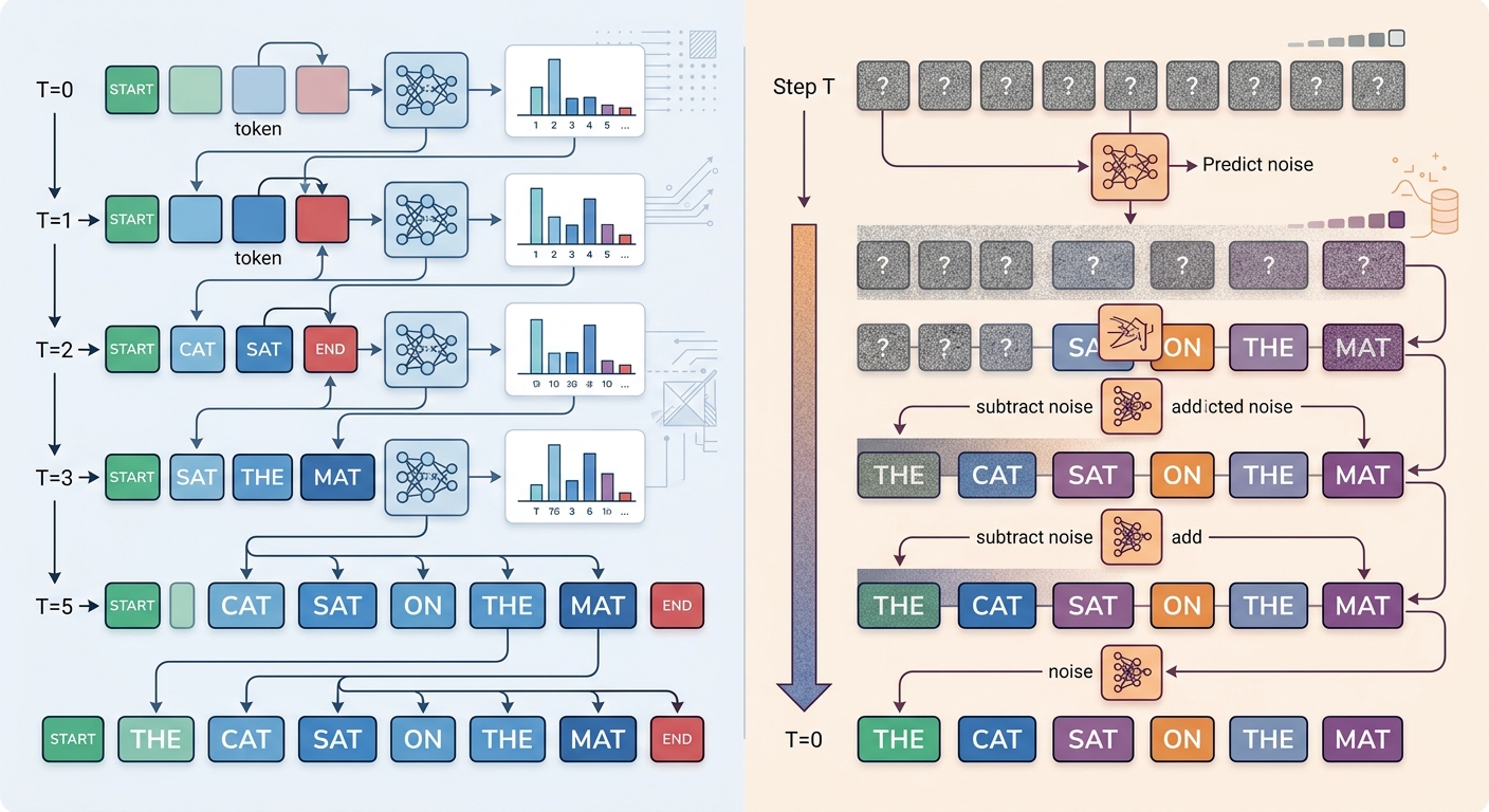
An AR model computes the probability of each token conditioned on every prior token. Generation is inherently sequential: emit token n, feed it back, emit token n+1. The KV-cache makes this tractable by storing past attention states, but the loop itself is the bottleneck. Total latency scales roughly linearly with output length, and every token depends on the one before it. This is why AR serving stacks obsess over batching, speculative decoding, and cache management — they're all workarounds for a fundamentally serial process.
The serial loop has a second-order cost: tail latency. Because each request's completion time is a function of its own output length, a serving cluster mixes short and long generations, and the long ones dominate your p99. Continuous batching and paged attention (the core innovations behind vLLM and TensorRT-LLM) help by packing more requests onto each GPU step, but they don't change the underlying math — a 2,000-token response takes roughly 2,000 sequential decode steps no matter how you schedule it. (See our LLM inference optimization guide for the full serving-stack playbook.)
There's a subtlety worth naming because it drives the throughput comparison later: single-stream AR decode is memory-bandwidth-bound, not compute-bound. Each decode step reads the full model weights and KV-cache to produce one token per request. That's why batching is so effective for AR — one weight read serves many requests at once, so throughput scales well even though per-request latency doesn't improve much. AR's weakness is serial depth; its strength is that batching hides the cost of that depth across many requests.
Diffusion for text: iterative denoising over the full sequence
Diffusion models start from noise or a fully masked sequence and refine the whole thing over N steps. Each step updates many token positions in parallel, so the sequence emerges globally rather than left-to-right. Two families matter in practice: continuous diffusion, which operates in embedding space and projects back to tokens, and masked (discrete) diffusion, which progressively unmasks tokens. Masked diffusion has gained the most traction for text because it maps cleanly onto infilling and editing tasks. The math differs; the operational consequence is the same — generation is a bounded number of refinement passes over the full sequence, not a per-token loop.
A few mechanics are worth knowing because they drive the tradeoffs later. In masked diffusion, you choose a schedule — how many tokens to unmask per step, and whether to unmask highest-confidence positions first. Confidence-based unmasking (the low-entropy-first strategy from the Mask-Predict line of work, and the approach used in modern masked diffusion models like LLaDA and MDLM) tends to produce better quality than random unmasking, because easy tokens get locked in early and hard tokens get more refinement passes. Continuous diffusion models instead add noise to embeddings and learn to reverse the process, which gives smoother interpolation but requires a rounding step that can introduce artifacts. The practical upshot: masked diffusion is the family most teams will actually deploy for text, and its knobs — step count, schedule, and remasking policy — are the levers you'll tune. (Compare this with masked language modeling fundamentals if you're new to the paradigm.)
One mechanic deserves emphasis because it's the source of diffusion's control advantages: remasking. Because the model scores confidence per position at every step, it can revisit and replace tokens it locked in too early. That's the basis for constrained generation (force a schema-valid token, then let the rest reflow), infilling (condition on both left and right context), and edit-style tasks where the output must satisfy global constraints rather than a left-to-right commitment.
The practical consequence: sequential depth vs parallel width
AR cost scales with output length sequentially — serial depth. Diffusion cost scales with the number of denoising steps and the sequence length per step — parallel width. Both scale with length; the difference is in how the work is exposed to the hardware. AR trades depth for the ability to batch cheaply. Diffusion trades width for more FLOPs per generated token but exposes more parallelism within a single sequence.
That single difference drives almost every tradeoff below, and it determines which regime each architecture favors:
- Low batch, latency-sensitive (single user, interactive): diffusion's parallel width can cut wall-clock latency, because it doesn't pay N sequential steps for N tokens.
- High batch, throughput-sensitive (bulk offline jobs): AR usually wins on cost-per-token, because batching amortizes its per-step weight reads extremely well, while diffusion's extra FLOPs per token don't amortize as cleanly.
The two architectures also fail differently. AR degrades gracefully on latency — a slow request is just slow — but it can still fail on quality under aggressive quantization, context truncation, or speculative-decoding acceptance errors. Diffusion fails on quality if you cut steps too aggressively: you get a fast answer that's subtly wrong, which is often worse than a slow one that's right. Its saving grace is that the failure is tunable — step count and remasking are explicit knobs — whereas AR's quality regressions tend to be diffuse and harder to isolate.
Where Autoregressive LLMs Win
Output quality and instruction-following at the frontier
The frontier quality gap is still real — as of early 2026. Every major production frontier model setting records on open-ended reasoning, long-horizon instruction-following, and multi-step tool use is autoregressive. Years of scaling laws, RLHF pipelines, and data curation have been tuned for AR training dynamics. Diffusion models produce competitive text on constrained and structured tasks, and research models in the LLaDA and Mercury class are closing on narrow benchmarks, but on open-ended reasoning and nuanced instruction adherence, AR remains the quality reference point. If your workload tolerates zero quality regression, this alone often decides it. Treat this as a dated snapshot, not a permanent law — the gap is narrowing and worth re-benchmarking each cycle.
The gap is widest on tasks that require long chains of dependent reasoning — multi-step math, agentic tool use, code that must compile against a large context. These tasks reward the left-to-right inductive bias because each token genuinely depends on the last, and the model can "commit" to an intermediate result before building on it. Diffusion's global refinement is a strength for editing but is less proven on deep sequential dependency chains, where the error-recovery mechanisms (remasking, extra steps) add compute without a clean guarantee of correcting a poisoned intermediate. (For workloads like these, see our guide to reasoning model selection.)
Ecosystem maturity: tooling, fine-tuning, serving stacks
The AR ecosystem is a decade deep: vLLM, TensorRT-LLM, quantized serving, LoRA and full fine-tuning recipes, eval harnesses, observability integrations. Diffusion LLM tooling is improving fast but remains thinner — fewer production-grade serving runtimes, less mature quantization and batching support, and fewer battle-tested fine-tuning recipes. For a team that needs to ship in a quarter, the AR path has fewer unknowns and a larger hiring pool. Ecosystem maturity is not a quality argument, but in B2B infrastructure it is frequently the deciding one.
Where Diffusion Language Models Win
Latency under low batch and strict time-to-first-complete-token
The clearest diffusion win is the regime AR handles worst: low concurrency, hard latency budgets, and outputs long enough that N sequential decode steps dominate. Because diffusion refines the whole sequence in parallel, a single interactive request can complete in far fewer wall-clock steps than the equivalent token count under AR — provided step count is tuned low enough and quality holds. This is a real advantage for interactive UIs, voice, and agent steps where a single user is waiting.
Infilling, editing, and structured/constrained generation
Masked diffusion's native ability to condition on both sides of a span and to remask makes it a natural fit for fill-in-the-middle code completion, document editing, and generation under hard structural constraints (schemas, grammars, fixed formats). You can force a token and let the rest of the sequence reflow around it — something AR models approximate with constrained-decoding hacks but don't do natively. If your workload is "produce output that must satisfy global constraints," diffusion is worth a serious look.
Throughput and cost when step count is small
When quality tolerates a small number of denoising steps, diffusion can deliver high tokens-per-second per GPU on workloads where per-sequence parallelism matters more than batch amortization. The caveat is explicit: this is a quality-versus-steps tradeoff, and the win evaporates if you need many steps to hit your quality bar. Benchmark steps-to-quality on your own data before assuming the throughput advantage transfers.
Decision Matrix: Matching Architecture to Workload
| Workload signal | Autoregressive | Diffusion |
|---|---|---|
| Open-ended reasoning, long dependency chains | Strong | Weak (unproven) |
| Zero-tolerance quality regression | Strong | Risky |
| High-batch offline throughput, cost-per-token | Strong | Usually weaker |
| Low-batch, strict interactive latency | Weaker | Strong |
| Infilling / fill-in-the-middle | Adequate | Strong |
| Hard structural / schema constraints | Adequate (constrained decoding) | Strong (native) |
| Ecosystem, tooling, hiring | Strong | Thinner |
| Tunable quality/latency knobs | Limited | Strong |
How to Decide: A Practical Evaluation Protocol
- Define the failure mode you can afford. Slow-but-correct versus fast-but-subtly-wrong. This frames everything else.
- Benchmark steps-to-quality on your own data. For diffusion, sweep step count and schedule; find the floor where quality holds. Don't trust headline numbers.
- Measure at realistic concurrency. Diffusion's latency edge is a low-batch phenomenon; AR's throughput edge is a high-batch one. Test at your actual batch profile, not a demo.
- Price the ecosystem tax. Serving, quantization, fine-tuning, and observability maturity are real costs. Budget for them, not just tokens.
- Re-benchmark each cycle. The frontier quality gap is a moving target; a decision that was correct in early 2026 may not hold a year later.
The architecture choice is a bet on which failure mode your product can tolerate and which workload regime dominates your bill. Match the bet to the workload, not the hype.