Building Your First RAG Pipeline: A Step-by-Step Implementation Guide

When a legal team asks their LLM about a specific contract clause and the model confidently cites a provision that doesn't exist, the problem isn't the model — it's that the model was trained on public data and has never seen that contract. Retrieval-Augmented Generation fixes this by giving the LLM a retrieval step: find the relevant documents first, then generate an answer grounded in those documents.

RAG — Retrieval-Augmented Generation — combines a retrieval system with a language model. The retriever finds relevant context from a private corpus. The language model generates an answer using that context as a grounding source. By end of this article, you'll understand the full RAG pipeline architecture and have working Python code for each component, from document loading through LLM generation.

---

What Is RAG and Why It Matters in 2026

RAG has three core components. The index stores your documents in a searchable format — typically a vector database. The retriever takes a user query and finds the most relevant documents from the index. The generator — an LLM — produces an answer using the retrieved context. The result is a system that answers questions about your specific data, not just what the LLM saw during training.

RAG became critical as enterprise AI adoption accelerated through 2024 and 2025. Organizations realized that fine-tuning a model on their data was expensive, slow, and didn't solve the hallucination problem — a fine-tuned model still hallucinates about information it wasn't trained on. RAG provides a different trade-off: less expensive than fine-tuning, faster to implement, and fundamentally more honest because the model can only answer from retrieved documents.

The three primary approaches to customizing an LLM for private data are:

• Prompt engineering — cheapest, fastest, least reliable. Works for well-defined tasks with short context windows.
• Fine-tuning — improves task-specific behavior and reduces token usage. Does not solve hallucination on unseen documents. Expensive and slow to iterate.
• RAG — grounds answers in retrieved context, eliminates hallucination on private data, easy to update when data changes. Becomes the default choice for any application where data freshness or accuracy on private documents matters.

Does your data change frequently? If yes, choose RAG — you update the index without retraining. If your data is stable and you need consistent task behavior, fine-tuning may be appropriate. For most enterprise AI applications in 2026, RAG is the right starting point.

---

RAG Pipeline Architecture

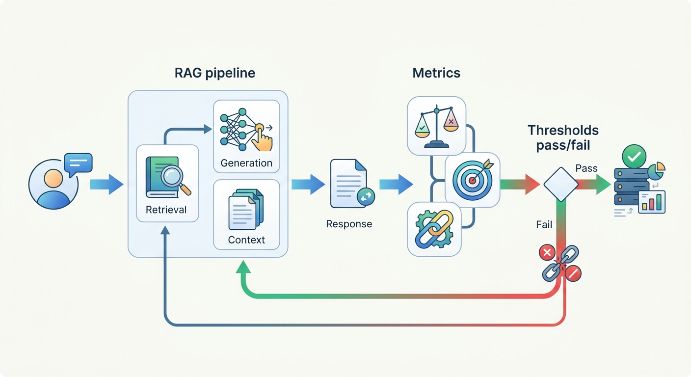
The RAG pipeline flows through seven distinct components. Here's how they connect:

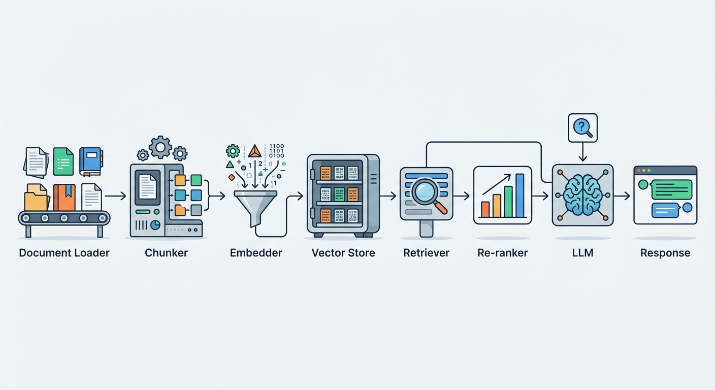
Document Loader ingests raw source files — PDFs, HTML pages, database records, Slack exports, Confluence dumps. Each format requires a specialized loader. A PDF loader extracts text while preserving page structure and headings. An HTML loader strips markup and extracts clean text content.

Chunker splits documents into smaller pieces — typically 512 to 2,048 tokens. Chunk size is a critical tuning decision: too small and you lose context; too large and you introduce noise or exceed your model's context window.

Embedder converts each chunk into a dense vector embedding — a list of floating-point numbers that represents the semantic meaning of the text. The same text always produces the same embedding. Semantically similar texts produce similar vectors.

Vector Store indexes these embeddings for fast similarity search. When a query comes in, you embed the query and find the k nearest vectors — the k most semantically similar chunks.

Retriever executes this search and returns the top-k results. This is where your pipeline's quality lives or dies: a good retriever finds exactly the chunks that answer the user's question.

Re-ranker (optional but recommended) applies a more expensive cross-encoder model to reorder the retrieved chunks. Vector similarity is fast but imperfect; a re-ranker evaluates query-document relevance more deeply and often changes which chunks should be prioritized.

LLM receives the original query plus the retrieved context and generates an answer. The retrieved context dramatically reduces hallucination because the model can only reference documents it has been given.

---

Document Ingestion and Chunking

The ingestion pipeline prepares your raw documents for retrieval. Here's a typical implementation:

from langchain_community.document_loaders import PyPDFLoader
from langchain.text_splitter import RecursiveCharacterTextSplitter

loader = PyPDFLoader("annual-report-2025.pdf")
documents = loader.load()

chunker = RecursiveCharacterTextSplitter(
    chunk_size=1024,      # tokens per chunk
    chunk_overlap=128,    # overlap between chunks
    separators=["\n\n", "\n", ". ", " "]
)
chunks = chunker.split_documents(documents)

Chunk size directly affects retrieval quality. The right size depends on your use case.

Use Case	Chunk Size	Overlap	Rationale
Code search	256–512 tokens	64 tokens	Function-level retrieval; larger loses precision
Legal documents	1,024–1,536 tokens	128 tokens	Preserve clause context; sentences are long
Technical documentation	512–1,024 tokens	128 tokens	Balance precision with coverage
Long-form articles	1,024–2,048 tokens	256 tokens	Preserve paragraph and section context
Q&A / FAQ	256–512 tokens	32 tokens	Single factual answer per chunk

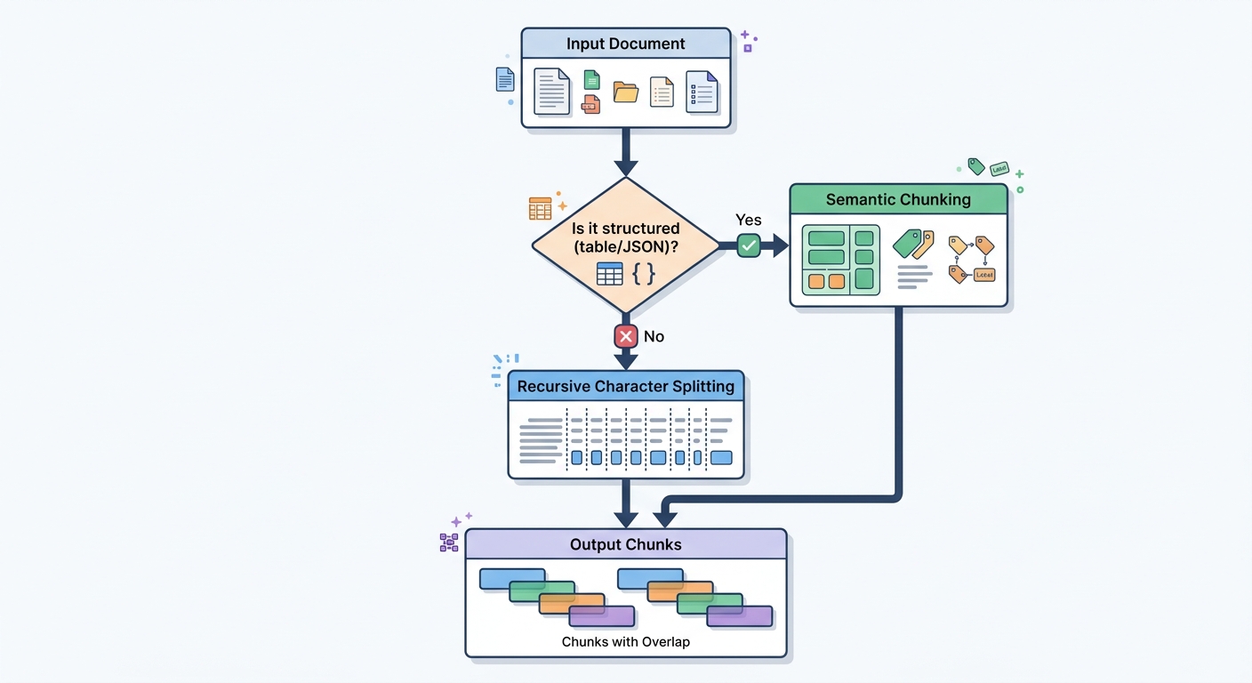
Recursive character splitting — as shown above — tries to split on paragraph breaks first, then sentence breaks, then word breaks. This preserves semantic coherence better than fixed-size slicing, which might cut mid-sentence or mid-paragraph.

Structured data — tables, JSON, code — requires special handling. A table split naively across chunks becomes unreadable. Use specialized loaders that serialize tables to markdown or JSON strings as single units. For code, split on function or class boundaries rather than character count.

---

Embedding and Vector Storage

Embedding model selection matters more than most practitioners expect. A mediocre embedding model produces poor retrieval even with perfect chunking. ¹

Embedding Model	Dimensions	Context Length	Best For
OpenAI text-embedding-3-large	3,072	8,192 tokens	General purpose; best overall quality
Cohere embed-v4	1,024	512 tokens	Multilingual; fast inference
BGE-m3	1,024	8,192 tokens	Open-source; competitive quality
E5-mistral-7b	1,024	4,096 tokens	Highest accuracy; slower inference

For most production applications, text-embedding-3-large or BGE-m3 are the right defaults. OpenAI's model has the best overall accuracy; BGE-m3 is the open-source alternative at comparable quality.

The vector database stores your embeddings and serves similarity searches. The choice affects scalability, latency, and operational complexity. ²

Vector DB	Deployment	Scalability	ANN Algorithm	Best For
Pinecone	Managed cloud	Excellent	Proprietary	Production at scale; minimal ops
Weaviate	Cloud or self-hosted	Excellent	HNSW	Hybrid search (vector + BM25)
Chroma	Local / embedded	Moderate	HNSW	Prototyping; small-scale production
FAISS	Self-hosted	Excellent	HNSW / IVF	Large-scale self-hosted; cost control

For teams starting out, Chroma is the fastest path to a working pipeline. For production at scale, Pinecone or Weaviate handle hundreds of millions of vectors with sub-100ms p99 latency.

import chromadb
client = chromadb.Client()
collection = client.create_collection("rag-docs")

# Add chunks with metadata
collection.add(
    ids=[f"chunk-{i}" for i in range(len(chunks))],
    embeddings=embeddings,       # list of float vectors
    documents=[c.page_content for c in chunks],
    metadatas=[{"source": c.metadata.get("source", "unknown")} for c in chunks]
)

---

Retrieval Optimization

Basic retrieval — embed the query, find top-k by cosine similarity — works for demos. Production pipelines need more.

Maximum Marginal Relevance (MMR) retrieves chunks that are both relevant to the query and diverse from each other. Without MMR, you might retrieve five chunks that are all from the same section of the same document — redundant coverage, missing perspective.

Query expansion transforms a short user query into multiple reformulations, retrieves against all of them, and deduplicates. A query like "How does the model handle PII?" becomes: ["How does the model handle PII?", "What is the data privacy approach?", "PII processing in the system"]. Retrieval across all three variants produces more comprehensive coverage.

HyDE (Hypothetical Document Embeddings) generates a hypothetical answer to the query, embeds that answer, and retrieves documents similar to the hypothetical answer. The intuition: documents that would support a correct answer are better retrieval targets than documents that literally contain the query terms.

Hybrid search combines dense vector similarity with sparse keyword search (BM25). This catches cases where the query contains specific terms — product names, IDs, technical jargon — that semantic embedding might not weight heavily enough.

---

Re-Ranking: Retrieving the Right Chunks

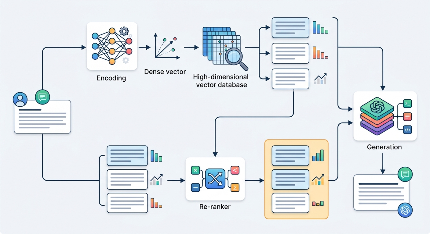
Vector similarity search is fast but semantically limited. A cross-encoder re-ranker evaluates the full query-document relationship more deeply, at the cost of higher compute.

Bi-encoder retrieval (standard vector search) embeds the query and document independently, then compares vectors. Fast, scalable, but loses fine-grained interaction between query terms and document content.

Cross-encoder re-ranking takes the query and document together through a transformer model and outputs a relevance score. More accurate, but too expensive to run on millions of documents — so you run it only on the top 50–200 candidates from the bi-encoder stage.

Open-source re-ranker options include BGE Reranker and Cohere Rerank (API). In practice, adding a re-ranker to a RAG pipeline typically improves answer quality by 10–20% on domain-specific queries. The cost is a 20–50ms latency addition per query — acceptable for most production applications.

---

Generation with LLM

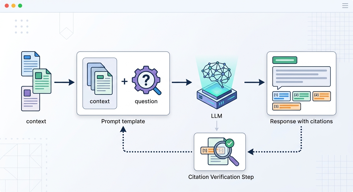
The LLM receives a prompt that includes the user query and the retrieved context. The quality of this prompt determines how faithfully the model uses the retrieved context. ³

LLM	Context Window	Strengths	Weaknesses
GPT-4o	128K tokens	Best reasoning; strong citations	Cost per token
Claude 3.5 Sonnet	200K tokens	Long context handling; instruction following	Slightly lower factual precision than GPT-4o
Llama 3.1 70B	128K tokens	Open-source; cost-effective self-hosting	Requires more prompt engineering
Mistral Large 2	32K tokens	Fast inference; strong European data compliance	Smaller context window

For most production RAG applications, GPT-4o or Claude 3.5 Sonnet are the appropriate defaults. Both produce reliable citations and handle ambiguous queries gracefully. Llama 3.1 70B is the right choice when data privacy requirements demand self-hosted deployment.

Prompt templating best practice: always include an instruction to cite sources and a placeholder for the retrieved context. A minimal effective answering prompt:

You are a helpful assistant. Use the provided context to answer the question.
If the answer is not in the context, say so clearly. Cite the source(s) you used.

Context: {retrieved_chunks}

Question: {user_query}

---

Evaluating Your RAG Pipeline

RAG evaluation answers one question: is the system giving accurate, grounded answers? Three RAGAS metrics are the standard:

• Context Precision — of the retrieved chunks, what fraction is actually relevant to the question? High context precision means low noise in retrieved results.
• Faithfulness — does the generated answer stay faithful to the retrieved context? Low faithfulness means the model is adding information not present in the retrieved documents.
• Answer Relevancy — does the generated answer directly address the user's question? High answer relevancy means the system understood what was being asked.

Synthetic evaluation — generating test question-answer pairs from your documents automatically — is the practical approach for most teams. Use an LLM to generate 50–200 question-answer pairs from your corpus, run your RAG pipeline against those questions, and measure RAGAS scores. A score below 0.7 on Faithfulness is a production red flag — the model is adding information beyond what the retrieved documents contain.

Common failure modes:

• Noisy retrieval — irrelevant chunks polluting the context window. Diagnose by checking context precision; fix by tuning chunk size, improving embedding model, or adding a re-ranker.
• Context overflow — too many chunks exceed the model's context window. Fix by reducing top-k or compressing retrieved chunks.
• Stale embeddings — index is out of sync with documents. Fix by rebuilding the index on a schedule or triggering rebuilds on document updates.

---

Production Considerations

Moving from prototype to production requires addressing five concerns that demos ignore.

Latency. Users expect answers in under three seconds. Target a p95 latency of under 2,000ms end-to-end. Chunk your pipeline: retrieval should complete in under 200ms (FAISS HNSW at 1M vectors achieves this), re-ranking in 20–50ms, generation in 500ms–1,500ms depending on model and output length.

Cost control. Embedding ingestion is a one-time cost per document. Retrieval and generation are per-query costs. Cache query embeddings for repeated or semantically similar queries — a 30–50% cache hit rate reduces retrieval costs significantly. Monitor cost per 1,000 queries and set alerting thresholds.

Security and data isolation. If you're using an external LLM API, confirm your data is not used for training. For highly sensitive documents, use a self-hosted LLM or a provider with explicit data isolation guarantees (Anthropic, for example, does not train on API data by default).

Index freshness. Document updates require re-embedding and re-indexing. Implement an incremental update pipeline that processes only changed documents, not the entire corpus. Set up monitoring for embedding drift — a gradual increase in retrieval latency or a drop in context precision often indicates the index is stale.

Monitoring. Log every query, retrieved chunk set, generated answer, and user feedback signal. Track answer faithfulness over time — a declining Faithfulness score is an early warning that your retrieval is degrading.

---

Framework Comparison: LlamaIndex vs LangChain vs Haystack

Framework	Strengths	Weaknesses	Best For
LlamaIndex	RAG-first design; excellent retrieval primitives; clear data framework	Smaller ecosystem than LangChain	Teams building RAG as primary use case
LangChain	Broad AI app framework; agent support; large community	Complexity overhead; steeper learning curve for RAG specifically	Teams building broader AI applications (agents, chains, tools)
Haystack	Strong for production-scale pipelines; OpenSource-first; good Kubernetes support	Smaller community; fewer third-party integrations	Teams on Python who want production-scale self-hosted

For teams building a RAG pipeline as their primary AI application, LlamaIndex is the right starting point — its design philosophy is retrieval-first and its documentation is oriented around RAG use cases. For teams building broader AI-powered applications with agents, tool use, and multi-step reasoning, LangChain offers more flexibility. Haystack is the choice for teams committed to self-hosted, open-source infrastructure at scale.

---

Conclusion

A production-ready RAG pipeline has five core stages: load your documents, chunk them to the right size for your use case, embed and index them in a vector database, retrieve relevant chunks with query optimization and re-ranking, and generate answers grounded in that context. Each stage has tuning decisions that significantly affect answer quality.

Start with one data source, implement the full pipeline end-to-end, and evaluate with RAGAS metrics before adding complexity. Most pipeline failures trace to one of three issues: wrong chunk size, weak embedding model, or insufficient retrieval evaluation. Fix those before scaling to more documents or adding multi-step reasoning.

Algorithmine's AI integration team helps enterprises design, implement, and evaluate RAG pipelines — from data ingestion architecture through production monitoring and cost optimization. Teams building their first RAG system can schedule a no-commitment architecture review.

---

Frequently Asked Questions

What is the difference between RAG and fine-tuning?

RAG retrieves relevant documents at query time and uses them as context for generation. Fine-tuning updates the model's weights on a specific dataset, changing how the model behaves across all queries. RAG is better for data that changes frequently and for grounding answers in specific documents. Fine-tuning is better for improving task behavior (tone, format, reasoning style) on stable data.

What chunk size should I use for RAG?

512–1,024 tokens is the right default for most use cases. Code search works better at 256–512 tokens (function-level precision). Long legal or technical documents benefit from 1,024–2,048 tokens to preserve section context. Always experiment: a 20% change in chunk size can improve or degrade answer quality by 10–15% on domain-specific queries.

How do I evaluate a RAG pipeline?

Use RAGAS metrics: Context Precision (relevance of retrieved chunks), Faithfulness (does the answer stay within retrieved context?), and Answer Relevancy (does the answer address the question?). Generate synthetic question-answer pairs from your documents and measure these scores. Faithfulness below 0.7 in production is a red flag that the model is hallucinating beyond the retrieved context.

What is a vector database and why do I need one?

A vector database indexes document embeddings for fast similarity search. When a user query comes in, the vector database finds the k most semantically similar chunks in milliseconds — something a standard relational database cannot do efficiently. Without a vector database, retrieval at query time would be too slow for production use.

How does retrieval optimization improve RAG quality?

Basic top-k retrieval by cosine similarity often returns redundant or noisy chunks. Retrieval optimization techniques — MMR for diversity, query expansion for better coverage, HyDE for intent-aware retrieval, hybrid search combining vector and keyword matching — collectively improve context precision by 15–30% compared to naive retrieval. Adding a re-ranker improves it further.

Can RAG work with structured data like tables and JSON?

Yes, but structured data requires special handling. Tables should be serialized as markdown or JSON strings rather than split across chunks. A table split naively will become unreadable in a RAG context. For JSON data, extract the relevant fields and embed them with sufficient surrounding context. Code should be split on function or class boundaries, not character count.

---

Expert Q&A: RAG Pipeline Implementation

Q: Why does naive cosine similarity retrieval often miss the most relevant chunks on domain-specific queries, and what is the actual mechanism by which hybrid search fixes it? A: Bi-encoder embedding models compress semantic meaning into dense vectors, but they lose term-level precision in the process. A query like "GDPR Article 17 right to erasure" gets embedded into a dense vector that captures semantic intent well — but it may not match vectors from a document that literally says "Article 17 — Right to Deletion" if the embedding model wasn't specifically fine-tuned on legal terminology. Hybrid search solves this by combining dense vector similarity (capturing semantic similarity) with BM25 sparse retrieval (capturing exact lexical matching). The BM25 component catches the specific article numbers, section names, and technical terms that dense embeddings underweight. The vector component catches semantically similar paraphrases. Combining both scores with reciprocal rank fusion (RRF) outperforms either method alone by 15–25% on domain-specific corpora, which is why production RAG pipelines consistently adopt hybrid search once they move beyond generic data.

Q: What is the most commonly overlooked production failure mode in RAG pipelines, and how does it present before causing visible answer quality degradation? A: Embedding model degradation is the silent failure mode most teams miss. An embedding model that worked well on your initial corpus begins producing worse vectors as your document composition changes over time — new product categories, different writing styles, updated terminology. The retrieval still runs, top-k chunks still return, and the system appears functional. The degradation only surfaces when you notice answer quality dropping in production or when Faithfulness scores on your evaluation set decline gradually over weeks. The fix is systematic: run retrieval evaluation on a fixed benchmark set monthly, track retrieval precision over time, and trigger a re-embedding pipeline when you add major new document categories or when evaluation metrics decline 10% or more from baseline. Treating your embedding model as a static component is the mistake — it needs the same observability treatment as your retrieval pipeline itself.

Q: How should teams think about the trade-off between context window size and retrieval quality in 2026, given that leading LLMs now support 128K–200K token contexts? A: The intuition that larger context windows reduce the need for precise retrieval is misleading and expensive. Passing 50 retrieved chunks into a 128K context window doesn't improve answer quality — it dilutes the relevant context with noise, increases LLM inference latency proportionally, and raises per-query cost 3–5×. The retrieval precision floor stays the same: irrelevant chunks in the context still confuse the model. The practical approach is to keep chunk count modest (4–8 chunks for most use cases) and invest in retrieval quality — better embeddings, re-ranking, hybrid search — so that the chunks you retrieve are the highest-quality possible. Use large context windows for multi-document synthesis tasks where you genuinely need to reason across many documents simultaneously, not as a substitute for retrieval precision. The 200K context window is a backstop for complex reasoning, not a retrieval quality solution.

Footnotes

1. Internal link suggestion: Vector database comparison guide — deep-dive on Pinecone vs Weaviate vs Chroma for production RAG systems. ↩

2. Internal link suggestion: AI data integration services — architecture support for enterprise document processing and RAG pipeline design. ↩

3. Internal link suggestion: LLM integration consulting — production LLM deployment and prompt engineering for RAG applications. ↩