Feature Engineering at Scale: Automated Feature Selection for High-Dimensional Enterprise Data

Introduction

In 2026, enterprise machine learning teams face a familiar and growing problem: datasets are getting wider faster than they are getting deeper. A single enterprise dataset might contain hundreds of raw columns, thousands of one-hot encoded categoricals, dozens of embedding vectors generated from NLP or computer vision pipelines, and a smattering of behavioral aggregates computed over rolling time windows. The result is a feature space that can stretch into tens of thousands of dimensions and a model that chokes on the noise.

This is the curse of dimensionality, and it manifests in two concrete ways. First, model performance degrades as irrelevant and redundant features obscure the signal that actually matters. Second, training time and inference latency scale poorly with feature count, driving up compute costs in cloud environments where you pay per vCPU-hour. The solution is automated feature selection: a systematic, reproducible pipeline that identifies and retains only the features that genuinely contribute to predictive power.

This article walks through the three canonical families of feature selection methods — filter, wrapper, and embedded — and then drills into the techniques that modern enterprise ML teams rely on most: correlation filtering, recursive feature elimination (RFE), and SHAP-based importance ranking.

The Three Families of Feature Selection

Before diving into specific techniques, it helps to understand the taxonomy. All feature selection methods fall into one of three categories based on how they evaluate a feature's usefulness.

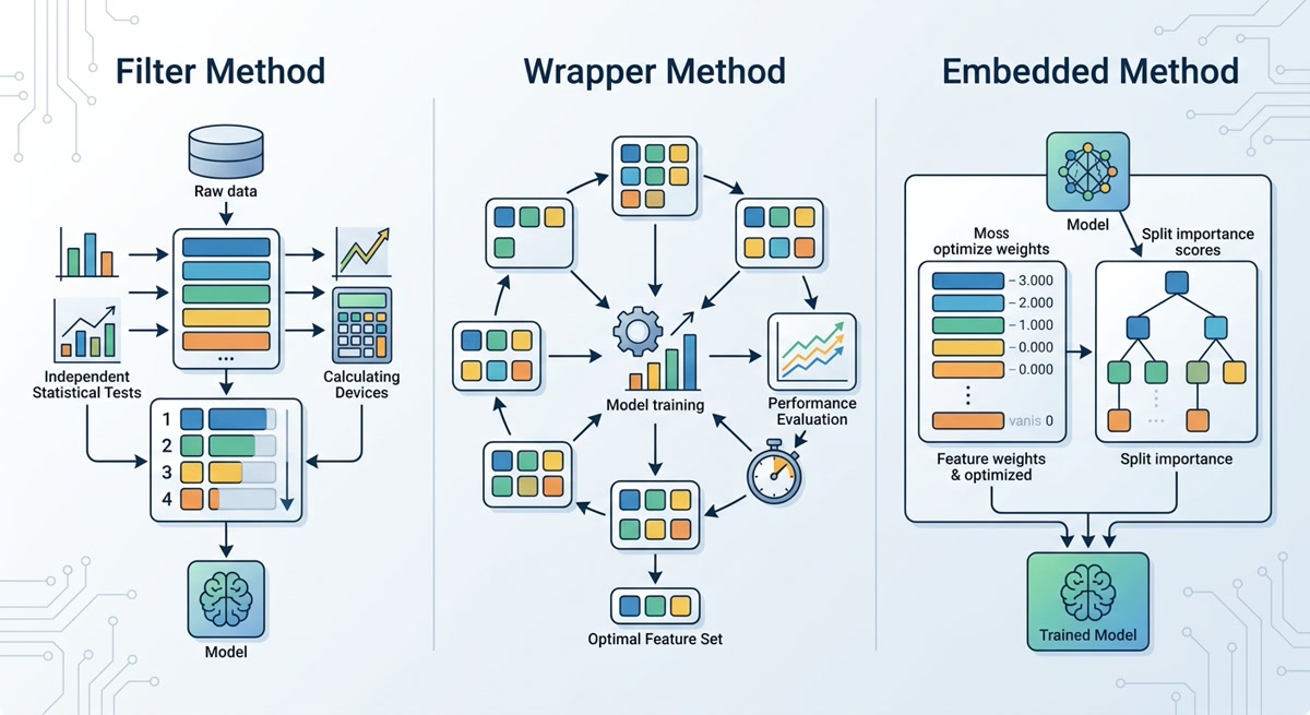
Filter methods apply a statistical test to each feature independently of any model. Common tests include chi-square for categorical targets, mutual information for capturing nonlinear relationships, and ANOVA F-value for continuous targets. Filters are fast because they require no model training, and they are model-agnostic, meaning the selected features will work with any downstream learner. Their weakness is that they cannot capture feature interactions — a feature that is useless on its own but powerful in combination with another will be incorrectly discarded by a univariate filter.

Wrapper methods evaluate feature subsets by training the actual model and measuring its performance. Forward selection starts with zero features and adds them one by one; backward elimination starts with all features and removes them one by one; and recursive feature elimination (RFE) removes the weakest features iteratively, retraining at each step. Wrappers can capture interactions because they measure the effect of features within the context of a model. The cost is computational: a full RFE run requires dozens or hundreds of model fits, which becomes prohibitive with thousands of features and large datasets.

Embedded methods perform feature selection during model training, making them more efficient than wrappers. In regularized linear models, L1 (LASSO) penalization drives coefficients to zero for irrelevant features, effectively performing selection as part of optimization. Tree-based models like XGBoost and LightGBM split on the most informative features at each node; the frequency and importance of splits provide a natural feature ranking. Embedded methods are the most widely used approach in production today because they combine the interaction-awareness of wrappers with the speed of filters.

Correlation Filtering: The First Line of Defense

When enterprise teams audit their feature spaces, they consistently find the same structural problem: redundancy. Derived features are often computed from the same base column. Rolling statistical aggregates — moving averages, exponential moving averages, standard deviations — are mathematically correlated with the raw values they are computed from. One-hot encoded categoricals generated from the same parent column are perfectly negatively correlated by definition. Failing to address this redundancy wastes model capacity on duplicate signals and inflates the apparent importance of features that are merely correlated with each other rather than with the target.

Correlation filtering addresses this systematically. The approach has three steps:

First, compute the pairwise correlation matrix across all numeric features. Second, convert the correlation matrix into a distance matrix and apply hierarchical clustering to identify groups of highly correlated features — features with a correlation coefficient above a threshold (typically |r| > 0.85 or |r| > 0.90 in enterprise contexts) are grouped together. Third, for each cluster, retain the feature with the highest variance or the strongest univariate relationship with the target, discarding the rest.

This approach is fast — computing a correlation matrix on a dataset with ten thousand features takes seconds in pandas with a modern BLAS library — and it is entirely model-agnostic. Libraries like feature-engine provide a DropCorrelatedFeatures transformer that automates the entire pipeline, including the dendrogram-cutting step.

Recursive Feature Elimination and Its Extensions

Once noise and redundancy are pruned with filters and correlation analysis, the next stage is to identify the features that have genuine predictive power in the context of a model. This is where recursive feature elimination (RFE) earns its place in any serious ML toolkit.

Classic RFE works as follows: train a model on the current feature set, compute a feature importance score, remove the bottom k features by importance, and repeat until the desired feature count is reached. RFE becomes far more powerful when combined with cross-validation. RFECV runs a full cross-validation sweep across all possible feature counts along the elimination path, revealing the exact feature count at which performance plateaus.

For enterprise pipelines in 2026, two extensions deserve special attention. Permutation importance shuffles each feature's values randomly and measures the resulting drop in model performance — model-agnostic and stable across multiple shuffles. SelectFromModel selects features whose importance exceeds a threshold, enabling one-shot selection without iterative elimination.

SHAP Values: Game-Theoretic Feature Importance

In 2026, the most powerful tool in the automated feature selection arsenal is not a specific algorithm — it is a framework. SHAP (SHapley Additive exPlanations) applies cooperative game theory to machine learning, computing each feature's marginal contribution to the model's prediction relative to a baseline.

The key property that makes SHAP superior to raw feature importance is local accuracy. A feature's SHAP value tells you, on average, how much that feature shifts the prediction away from the baseline. SHAP values are additive and locally accurate, meaning they can be aggregated meaningfully across the entire dataset and also decomposed for individual predictions.

For feature selection, the SHAP workflow is: compute SHAP values, rank features by mean absolute SHAP value, and select the smallest subset that cumulatively accounts for 95–99% of total SHAP importance. SHAP interaction values also reveal redundant feature pairs — high interaction between two features means they are not contributing independently.

Building an Automated Feature Selection Pipeline

The methods described above are most powerful when composed into a staged pipeline:

Stage 1: Domain and structural filtering — Remove constant columns, unique identifiers, and features with more than 95% missing values using VarianceThreshold.

Stage 2: Correlation deduplication — Hierarchical correlation clustering typically removes 20–40% of features in enterprise datasets.

Stage 3: Univariate statistical screening — Mutual information or ANOVA F-value to remove features with no univariate relationship to the target.

Stage 4: SHAP-based importance ranking — Select features at the 95% cumulative SHAP importance knee point.

Stage 5: RFECV validation — Confirm selection improves cross-validation performance.

Avoiding the Pitfalls

The most common failure mode is data leakage through feature selection. If you apply feature selection using the full training set before CV splits, validation scores will be optimistically biased. Fix: wrap feature selection inside the CV loop or use a held-out selection set.

Feature instability is a second pitfall. Robust pipelines run bootstrap or k-fold importance sampling and retain only features that appear in top-k across at least 80% of folds.

Over-reliance on univariate filters is third. Features that look weak in isolation can be powerful in combination — always follow filter methods with SHAP or RFECV.

Finally, selection without business logic can produce models that are technically sound but operationally broken. Audit every selected feature against production data availability constraints.

Conclusion

Automated feature selection is not optional for enterprise ML at scale — it is a prerequisite for models that are fast, interpretable, and robust. The most effective approach in 2026 combines fast model-agnostic filters with model-aware importance ranking in a staged pipeline. Start with correlation filtering and variance thresholding, validate with SHAP, and confirm with RFECV. The result is a leaner model that trains faster, generalizes better, and is far easier to debug and audit in production.