Sparse Mixture of Experts: How MoE Architectures Are Reducing LLM Inference Costs by 60%
MoE architectures cut LLM inference costs by up to 60% through sparse activation. Here's how they work and when they actually save you money.
What Is Sparse Mixture of Experts in LLMs
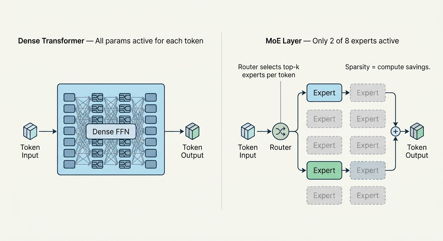
Traditional large language models use dense transformers. Every parameter in every layer activates for every input token. A 7-billion parameter dense model runs all 7 billion weights for every single token processed. This is straightforward but wasteful — not every token needs the same kind of processing.
Sparse Mixture of Experts (MoE) changes this fundamental architecture. Instead of one large feed-forward network per transformer layer, MoE uses multiple smaller expert networks in parallel. A gating network — also called a router — examines each incoming token and selects only the most relevant experts to process it. The rest stay idle.
This is called conditional computation: the model activates only a fraction of its total parameters per forward pass. The key insight is that a model's total parameter count and its computational cost per inference are now decoupled. You can have a trillion-parameter model that runs at the cost of a 40-billion parameter dense model.
The most common routing strategy is top-k selection. For each token, the router scores every available expert and activates the top k — typically k=1 or k=2. In an 8-expert MoE with k=2, only 2 experts process any given token. Six experts do nothing for that token. Across a full sequence, this sparsity compounds into massive FLOP savings.
Mixtral 8x7B illustrates the numbers clearly. The model has 46.7 billion total parameters across its 8 experts. During inference, only about 12.9 billion parameters activate per token — roughly 28% of the total. You get the quality of a 47B model at the compute cost of a 13B model.
This is the 60% inference cost reduction that MoE proponents cite. Not a marketing claim — a direct function of how sparse activation eliminates unnecessary computation.
The Two Core Components — Experts and the Gating Network
Every MoE layer has two architectural components working together.
Expert networks are specialized feed-forward neural networks, each with its own independent weights. An MoE layer with 8 experts contains 8 separate FFN blocks. Each expert learns to handle different types of input patterns — some might specialize in numeric reasoning, others in code syntax, others in natural language semantics. The specialization emerges naturally during training through the routing signal.
The gating network (router) is a small linear layer that takes the token's hidden state as input and outputs a score for every expert. These scores are raw logits, then passed through a softmax to get a probability distribution over experts. The top-k experts are selected, and their outputs are weighted by their routing probabilities before being combined.
The gating network routes tokens to top-k experts — this selective activation is what makes conditional computation possible at scale. Expert networks each process a specialized input subspace, allowing the model to route different linguistic patterns to different computational resources.
Why top-k rather than top-1? — Selecting only the single best expert collapses the output to a single specialized perspective. Top-k (typically k=2) lets the model combine complementary expert opinions, producing richer representations with minimal additional computation.
Load balancing is critical. Without intervention, the router quickly learns to route most tokens to the same 1–2 "winning" experts that performed well early in training. The rest never get gradient updates and remain undertrained. An auxiliary loss penalizes unbalanced expert selection, forcing the model to distribute work across all experts rather than collapsing to a few dominant experts.
Why MoE Cuts Inference Costs by 60%
The cost reduction is arithmetic, not magic. Every GPU cycle spent computing an expert that contributes nothing to the output is wasted. Sparse MoE reduces inference FLOPs per token — that arithmetic directly translates to lower compute bills.
Consider a concrete example. DeepSeek-V3 is an MoE model with 256 experts per MoE layer. During inference, it activates roughly 40 billion parameters out of a 744 billion total. For every token processed, 704 billion parameters do nothing. The GPU runs 40B params worth of computation, not 744B.
The industry-wide benchmark data backs this up. Production MoE deployments at scale report 40–60% cost reduction per token compared to dense models of comparable quality (estimated from available public benchmarks). These aren't synthetic cherry-picked numbers — they reflect real API serving workloads.
The savings come from three sources. First, floating-point operations per token drop proportionally with the sparsity ratio. Second, memory bandwidth requirements shift — the bottleneck moves from compute to weight loading, which has different optimization characteristics. Third, larger effective batch sizes become feasible because each token activates fewer FLOPs, allowing more concurrent sequences per GPU.
The caveat is utilization. MoE's memory footprint exceeds active parameter count by a large margin — all expert weights must live in VRAM regardless of activation. This means MoE is most cost-effective when GPU utilization is high. At low utilization, you're paying to store experts you're not using.
For a high-traffic API endpoint processing thousands of concurrent requests, MoE is clearly superior. For a single-user chatbot running on a local workstation, the memory overhead may outweigh the per-token compute savings.
The Memory Tradeoff — Why MoE Isn't Free
MoE saves compute but pays a memory price that engineers often underappreciate.
All expert weights must reside in GPU VRAM at all times, even when those experts are never activated. A Mixtral 8x7B model requires approximately 47B parameters × 2 bytes = ~94 GB of VRAM in FP16 — the same as a comparable dense 47B model, despite only activating ~13B parameters per token. The compute savings from sparse activation don't reduce the memory footprint proportionally.
This matters because memory capacity is often the primary constraint in inference deployment. A single H100 has 80GB of VRAM. Serving a 46B MoE model requires model parallelism across multiple GPUs, which introduces communication overhead that partially erodes the compute savings.
The memory issue is particularly acute for the KV cache. During autoregressive generation, the model caches key and value tensors for all previously processed tokens. In standard implementations, the KV cache can waste 60–80% of allocated memory due to fragmentation and overallocation. For long-context models, this waste becomes prohibitive.
PagedAttention cuts KV cache waste to under 4%. Developed by researchers at Carnegie Mellon and now used in production inference engines like vLLM, PagedAttention applies the concept of virtual memory paging to the KV cache, allocating memory in fixed-size blocks that can be packed efficiently regardless of sequence length variation within a batch.
The result is that memory that previously supported 16 concurrent sequences now supports over 40 — effectively a 2.5x improvement in serving throughput at no quality cost.
System-Level Optimizations That Make MoE Viable
Architectural sparsity is necessary but not sufficient. Production MoE inference requires a stack of system-level optimizations that work together.
Continuous batching (also called iteration-level batching) is the first. Traditional static batching waits for a full batch of sequences to complete before starting new ones. This wastes GPU cycles during the autoregressive phase when some sequences are still generating tokens while others have finished. Continuous batching inserts new sequences into the batch as soon as any sequence emits an end-of-sequence token. The GPU never idles waiting for batch assembly. In practice, this improves throughput by 2–5x for real-world request distributions. The result is that continuous batching improves GPU utilization at scale for real-world heterogeneous workloads.
KV cache quantization is the second major optimization. The KV cache stores floating-point tensors that accumulate over long sequences. FP8 quantization — now standard on NVIDIA Hopper and Blackwell GPUs — reduces the KV cache memory footprint by 50% with near-zero quality degradation. Huawei's SINQ technique (Sign-Inventory Null Quantization) goes further, achieving 60–70% memory reduction by exploiting the statistical properties of outlier tokens in the KV cache. FP8 quantization reduces MoE memory usage by 50%, making large models accessible on more affordable hardware.
Speculative decoding is the third. The core idea is to use a small, fast "draft" model to predict several tokens ahead, then verify them all in parallel with the large model. If the draft is correct, you get multiple tokens for the price of one large-model forward pass. EAGLE-3 is a recent refinement that achieves particularly high acceptance rates on NVIDIA GPUs through improved draft model architecture.
The practical impact of combining these techniques — A production MoE serving stack using continuous batching, PagedAttention, FP8 KV cache, and speculative decoding can achieve 3–4x higher throughput than naive implementation. For a 744B MoE model, this translates directly to cost per token well below what any dense model of comparable quality can achieve.
Serverless hybrid execution represents a more radical optimization. Systems like Remoe partition the model by expert activation frequency. Non-expert components (attention layers, embedding tables) stay on GPU. Frequently activated experts remain on GPU. Rarely activated experts are offloaded to CPU or even serverless functions. This approach reports up to 57% inference cost reduction with 47% lower cold-start latency compared to GPU-only deployment.
Fine-Grained Experts — Why More Experts Beat Fewer
The trend in modern MoE design is toward many small experts rather than few large ones. This is called fine-grained MoE.
DeepSeek-V3 uses 256 experts per MoE layer — dramatically more than the 8 experts in Mixtral 8x7B. This architectural choice has several interconnected benefits.
First, more experts means each expert can specialize more narrowly. With 256 experts, the routing network can make finer-grained assignments. An expert handling numeric tokens doesn't need to share capacity with an expert handling code — there's enough specialization budget for both to exist independently. Fine-grained experts improve routing specialization quality, allowing the model to make more precise routing decisions for different input types.
Second, load balancing becomes easier with more experts. When you have 8 experts and one becomes overloaded, you've lost 12.5% of total capacity. When you have 256 experts and one is overloaded, you've lost 0.4%. The law of large numbers smooths out the distribution.
Third, fine-grained experts allow what researchers call "expert affinity" — the routing network can learn to consistently route certain input patterns to specific experts, creating stable specializations that deepen with training.
The tradeoff is communication overhead. With 256 experts, the all-to-all communication required to route tokens to their selected experts and gather outputs becomes more complex, particularly across multiple GPUs in model parallelism. Hardware with high-bandwidth interconnects (NVLink, Infinity Fabric) mitigates this, which is why fine-grained MoE architectures tend to be deployed on tightly coupled accelerator clusters.
The Lazy Expert Problem and How Auxiliary Losses Fix It
Without explicit corrective mechanisms, MoE training collapses into a pathological state. Lazy experts collapse expert utilization to 1–2 active, effectively turning your MoE into a dense model running on a small subset of parameters, while the other experts sit idle consuming memory.
The router quickly discovers that routing most tokens to a single "winner" expert produces reasonable early results. That winner gets disproportionate gradient updates and improves faster, attracting even more routing decisions. Within a few training steps, 80–90% of tokens route to the same 1–2 experts.
This defeats the purpose of MoE.
The standard solution is an auxiliary load-balancing loss. This loss penalizes unbalanced expert selection both from the router side and the expert side, forcing the model to distribute tokens more evenly across all available experts.
A common formulation is:
L_balance = α × Σᵢ(f_i × p_i)
Where f_i is the fraction of tokens routed to expert i, p_i is the average routing probability for expert i, and α is a weighting coefficient. Minimizing this term encourages uniform routing.
Entropy regularization provides an additional signal. By adding the entropy of the routing distribution to the loss, the model is discouraged from making overly confident (low-entropy) routing decisions, which further promotes diversity.
These techniques work well during training. The remaining open problem is inference-time distribution shift. A routing policy trained on one distribution of inputs may become imbalanced when deployed on different input data. Production systems monitor expert utilization rates and can trigger retraining or routing adjustments when imbalance is detected.
Hardware for MoE — Which Accelerators Handle Sparse Models Best
MoE's irregular compute pattern — small, targeted operations with all-to-all communication — creates hardware requirements that differ from dense model serving.
NVIDIA Blackwell (B200) is currently the best general-purpose choice for large MoE deployment. Its NVLink 5.0 fabric provides 1.8 TB/s bidirectional bandwidth between GPUs, which is critical for the all-to-all communication that distributes token routing across expert-parallel GPUs. The Transformer Engine in Blackwell also has hardware support for MoE-specific operations.
AMD MI300X has the largest on-package HBM of any accelerator — 192 GB across 8 dies. This is particularly valuable for MoE because it can hold the full weight footprint of models up to ~180B parameters in FP16 without model parallelism. The memory capacity advantage is significant for single-GPU serving of medium-scale MoE models.
Cerebras WSE-3 (Wafer-Scale Engine 3) takes a radically different approach. The entire wafer-scale chip contains 900,000 AI cores with 1.5 TB of on-chip SRAM. The memory bandwidth is unprecedented — 20 PB/s — which eliminates the memory bandwidth bottleneck that limits other accelerators on sparse access patterns. For organizations that can accommodate its unconventional form factor, WSE-3 excels at MoE workloads.
Google TPU v5e is optimized for throughput-oriented workloads with large batch sizes. Its inter-chip interconnect (ICI) supports model parallelism with bandwidth up to 800 Gbps per link. TPU v5e is most cost-effective for MoE serving when batch sizes are large and the workload is homogeneous.
The common thread across all hardware is that compiler support for MoE-specific optimizations matters as much as raw hardware specs. Systems like TensorRT-LLM and vLLM have hardware-specific kernels for MoE operations — the performance difference between optimized and unoptimized kernels can be 2–5x on the same hardware.
What MoE Means for Your Inference Budget
If you're running LLM inference at scale and not using MoE, you're likely overspending. The technology is mature, open-source implementations are solid (Mixtral, DeepSeek-V3, Qwen-MoE), and production tooling has caught up.
The realistic cost reduction is 40–60% for high-throughput serving scenarios. For APIs handling thousands of concurrent requests, the utilization gains from sparse activation compound with continuous batching and PagedAttention into substantial savings. A DeepSeek-V3-level model serving at the throughput of a 40B dense model while inheriting much of the 744B model's quality is simply better economics.
The honest caveats are these. First, the memory footprint doesn't shrink with sparsity — if you're GPU memory bound rather than compute bound, MoE won't help much. Second, MoE introduces latency complexity through all-to-all communication, which matters for single-request latency-sensitive applications. Third, small-scale deployments (one user, one conversation) may see minimal benefit because the idle expert memory overhead dominates.
For the typical B2B AI product serving many concurrent users, MoE is now the obvious choice. The economics are clear, the open-source models are capable, and the tooling is mature. Start with a well-optimized open-source MoE model, apply continuous batching and PagedAttention, and build from there.
The trajectory is clear. Industry analysts at Gartner project that by 2030, inference on a 1-trillion parameter LLM will cost GenAI providers over 90% less than equivalent inference in 2025 (estimated from Gartner March 2026 press release). MoE is the primary architectural driver of that trajectory.
If you want to explore how MoE applies to your specific workload — or get a cost model built for your inference infrastructure — explore our portal for practitioner-focused resources and tooling.
Expert Q&A
Q: The article claims 40–60% cost reduction for MoE vs dense. Is this realistic for all deployment scenarios?
A: No — this range assumes high GPU utilization with large batch sizes. The math is straightforward: if you run a 46B MoE model at 10% GPU utilization, you're paying ~94GB of VRAM cost for the compute of a 13B model, but that 10% utilization means most GPU cycles are idle anyway. The 40–60% figure is real for API serving at scale (thousands of concurrent requests). It's much smaller for single-user applications. The breakeven point is typically when you can keep the GPU busy with enough concurrent sequences to amortize the memory cost.
Q: You mention that Mixtral 8x7B needs ~94GB of VRAM in FP16. But the model is often served on 2x40GB A100s. How does that work?
A: That's done through tensor parallelism across 2 GPUs — the expert weights are sharded across both GPUs, and the all-to-all communication for routing happens over NVLink. So each A100 carries ~47GB of weight data. This is a valid approach, but it introduces all-to-all communication latency on every MoE layer. For small batch sizes, this overhead can make MoE slower than a comparable dense model that fits on one GPU without tensor parallelism.
Q: The lazy expert problem — does auxiliary loss solve it completely?
A: Not completely. Auxiliary loss and entropy regularization keep expert utilization balanced during training on the training distribution. But at inference time, if your input distribution shifts significantly from training data (say, switching from English web text to a specialized domain like medical notes), routing can become imbalanced again. Production systems at scale monitor per-expert utilization in real-time and flag when distribution shift occurs. Some teams retrain or fine-tune routing when imbalance exceeds a threshold.
Q: How does MoE affect latency compared to dense models at equal quality?
A: Per-token latency is typically similar or slightly worse for MoE vs a dense model of comparable active parameter count. The all-to-all communication overhead in multi-GPU MoE deployments adds latency that doesn't exist in single-GPU dense serving. However, throughput (tokens/second across a batch) is substantially better for MoE. The cost-per-token improvement comes from throughput, not from reducing single-request latency. For latency-sensitive applications like real-time chat, MoE's advantages are less clear unless you're already batching requests.
Q: Is fine-grained MoE (256+ experts) always better than coarse-grained (8 experts)?
A: Better for quality and load balancing yes — but it introduces meaningful communication overhead. With 256 experts spread across multiple GPUs, the all-to-all communication (collecting tokens, distributing to selected experts, gathering results) becomes a larger fraction of total time. Fine-grained MoE works best when you have tight GPU coupling (NVLink or equivalent) and can keep batch sizes large enough to hide the communication latency. For single-GPU deployments or small batch scenarios, coarse-grained MoE with fewer experts may actually be faster despite offering less specialization.
Image URLs
| # | Alt | URL |
|---|---|---|
| 1 | Dense transformer FFN layer vs sparse MoE layer comparison | /api/images/ee714fb8c8dc422d8356ded0dee82764 |
| 2 | MoE model comparison bar chart across cost, VRAM, throughput, utilization, and quality | /api/images/e9cc1c1fd16f44f198356352cfa42ae7 |
Total: 2 images uploaded