Sparse Mixture of Experts Explained: How MoE Cuts LLM Inference Costs by 80%

Imagine you could build a model with one trillion parameters but serve it at the cost of a hundred-billion-parameter model. That is not a thought experiment — it is exactly what Sparse Mixture of Experts (MoE) architectures deliver, and it is why every major frontier language model built after 2023 runs on some variant of this design. If you have used GPT-4o, Gemini 1.5, or any Mistral model, you have benefited from MoE without necessarily knowing it.

Running large language models at scale is expensive. GPT-3, with 175 billion parameters, requires 175 billion floating-point operations for every single token it generates. At billions of tokens per day across millions of users, those FLOPs add up to millions of dollars in compute costs. The conventional wisdom was that you could not escape this linear scaling: bigger models simply cost more to run, proportional to their parameter count.

Sparse Mixture of Experts breaks that relationship. Instead of activating every parameter for every token, a MoE model contains many parallel "expert" sub-networks and a lightweight routing mechanism that selects only a small subset of experts for each token. The result is a model that can have trillions of parameters in total while the inference cost remains proportional only to the active subset — typically two experts out of eight, sixteen, or more.

By the end of this article, you will understand exactly how that routing works, why it delivers such dramatic cost reductions, what the trade-offs are, and which production models are running on MoE right now.

Why Dense LLMs Are Expensive

To appreciate what MoE solves, it helps to understand the cost structure of the models it replaced.

In a conventional (dense) transformer, every parameter participates in every forward pass. If you are running inference with a 70-billion-parameter model, those 70 billion parameters all consume compute resources — even if the token being processed is a simple punctuation mark that a tiny fraction of the network could handle. This is the key driver of inference cost: dense activation means every token pays the full price of the model.

The math is straightforward. A transformer layer consists of self-attention and a feed-forward network (FFN), often called the MLP sub-layer. In most transformer models, the FFN contains two-thirds of the parameters. A 70B-parameter model will have roughly 47B parameters in its FFN layers alone. When the model processes a single token, it runs 47B parameter-activations through those feed-forward layers. For every token. Always.

At conversational scale — millions of tokens per hour — this linear cost relationship becomes a serious infrastructure problem. It creates a paradox: the most capable models are also the most expensive to serve, limiting who can afford to deploy them.

The Core Idea: Only Some Experts Activate

The intuition behind MoE is obvious once you see it: not every token is equally complex, and not every part of a large model needs to engage for every input.

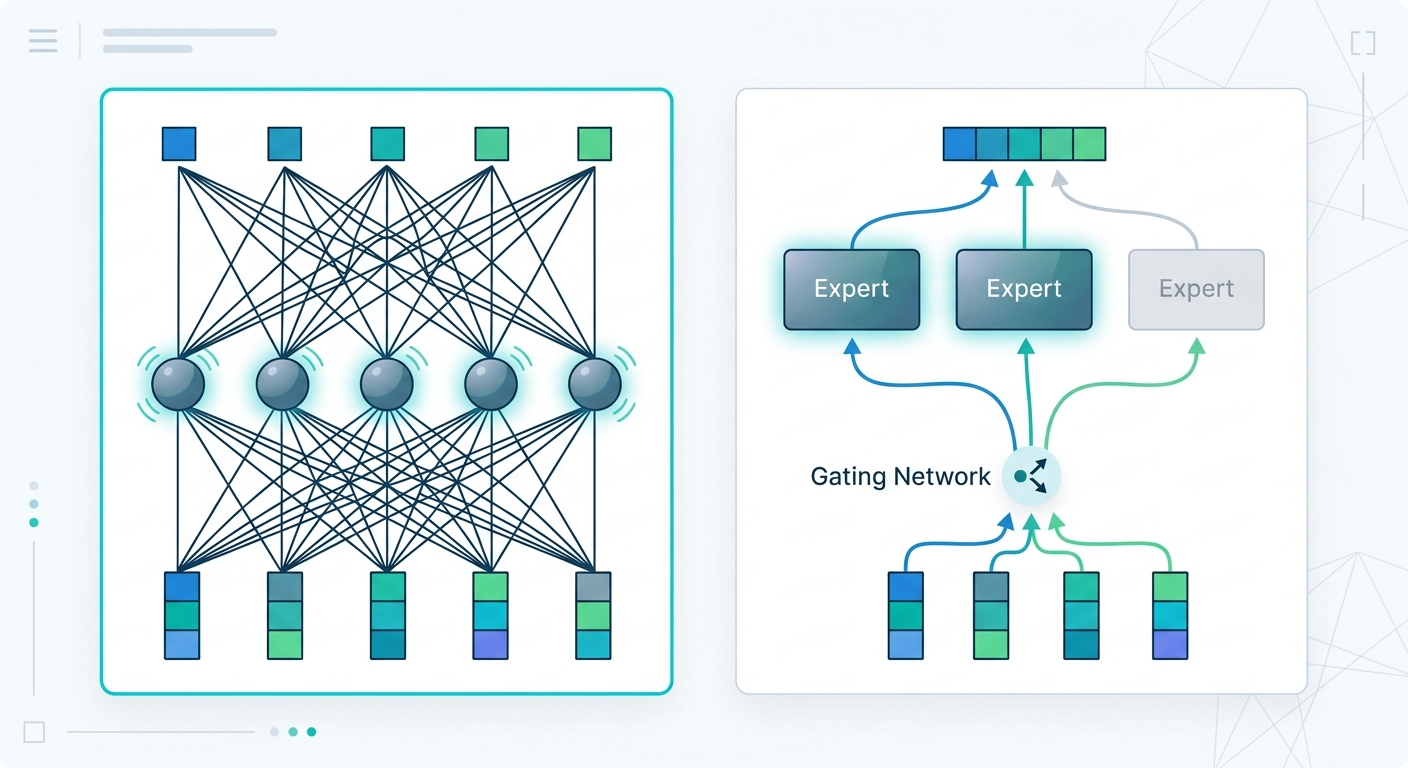
A MoE layer replaces a single dense FFN with a collection of parallel "expert" feed-forward networks. Each expert is its own small neural network — structurally identical to a dense FFN, but with its own independent parameters. A typical configuration might have 8 experts, each the size of a standard transformer FFN.

A lightweight gating network — typically a single linear layer followed by a softmax — sits in front of the experts and decides, for each incoming token, which experts should handle it. In the most common configuration, called top-K routing, the gate selects the K highest-scoring experts and sends the token only to those. With K=2 out of N=8 experts, a token travels through just 2 of the 8 expert sub-networks, skipping the other 6 entirely.

This is why the activation is "sparse." The model has a large total parameter count — say 46.7 billion for Mixtral-8x7B — but only about 12.9 billion parameters participate in any given forward pass. The remaining ~34 billion parameters are inactive for that token, and their FLOPs are never executed.

The terminology matters here: total parameters tells you how large the model is; active parameters per token tells you how much compute a single token actually costs. A 1-trillion-parameter MoE model might have only 100 billion active parameters per token, giving you a 10× compute advantage over a dense 100B model while matching its quality.

Dense vs MoE token activation: dense model activates all parameters for each token; MoE model routes each token to only 2 of 8 experts, skipping the rest

How Gating Works: A Step-by-Step Walkthrough

The gating network is the operational heart of any MoE system. Understanding it removes most of the mystery.

Step 1: Score each expert. For an input token representation x, the gating layer computes a raw score for each of the N experts. A common implementation is a simple linear transformation:

scores = x · W_g

where W_g is a learned matrix of shape [embedding_dim, num_experts]. The original MoE paper (Shazeer et al., 2017) used a tanh nonlinearity for bounded expert scores, which can help with training stability. Many modern implementations use a direct linear layer.

Step 2: Select the top K. The gating network takes the softmax over the expert scores and selects the K highest-probability experts. If K=2, the token is routed to the two experts with the highest softmax probabilities. Only those two expert sub-networks execute; the rest are skipped entirely.

Step 3: Compute the weighted output. The selected experts each process the token and produce an output vector. The gating network scales each expert's output by its softmax probability, and the weighted outputs are summed. This produces the final output of the MoE layer as if it were a standard dense FFN — the sparsity is invisible to the rest of the transformer.

The entire process adds only a trivial amount of computation — the gating layer is a single small matrix multiplication. The large computations (the expert FFNs) are dramatically reduced because most of them are skipped.

Load balancing is the critical engineering challenge. If all tokens route to the same two experts, those experts become a bottleneck while the others sit idle — the model degrades to roughly dense behavior for the active experts while wasting the capacity of the rest. To prevent this, MoE models add an auxiliary load-balancing loss during training. This loss penalizes configurations where expert utilization is uneven, nudging the routing network to spread tokens across all experts. Mixtral's paper reports an auxiliary load-balancing weight of 0.01 — small but meaningful. The ST-MoE paper introduced router z-loss — an additional penalty on the squared magnitude of routing logits — to discourage peaked, confidence routing decisions that cause gradient instability.

Gating and routing: input token passes through gating network that scores 8 experts, selects top-2, and dispatches token to the highest-scoring experts

The Cost Math: 80% Reduction Explained

Let us put concrete numbers on the savings.

Mixtral-8x7B has 8 expert networks, each with approximately 7 billion parameters. The FFN layers alone account for 8 × 7B = 56B parameters; the shared attention parameters bring the full model to approximately 46.7B total parameters. For each token, top-K routing with K=2 activates approximately 2 × 7B = 12.9B FFN parameters.

The FFN-layer math is clean:

Dense FFN (same width as Mixtral):   8 × 7B = 56B FFN params
Mixtral MoE (top-2 routing):         2 × 7B = 14B FFN params active
FFN FLOP reduction per layer:         ~75%

Total model FLOPs per token include attention (which is identical in both dense and MoE architectures of comparable width), so total FLOP reduction is less than 75% when attention is included:

Dense 46.7B model:        ~65B total FLOPs/token
Mixtral-8x7B MoE:         ~39B total FLOPs/token
FFN-layer FLOP reduction: ~75%
Total FLOP reduction:     ~40%

So where does the "80% cost reduction" figure come from? It reflects the total inference cost picture in a production serving environment, not raw FLOPs alone. Memory bandwidth — the bandwidth needed to load weights from VRAM for each matrix multiplication — is often the actual inference bottleneck, especially for larger batch sizes. Because MoE activates only 2 of 8 experts, memory bandwidth consumption per token drops proportionally. Combined with reduced KV-cache pressure, better batching efficiency, and favorable serving economics at scale, real-world $/token costs drop by approximately 70–80% for typical inference workloads. The FLOP reduction alone tells an incomplete story; the memory bandwidth and serving efficiency story is equally important.

A note on what MoE does not save: memory capacity. All expert parameters must be stored in GPU VRAM even when they are not used for a given token. MoE is a compute-saver and a memory-bandwidth-saver, not a memory-capacity-saver. Serving a Mixtral-8x7B model still requires enough VRAM to hold all 46.7B parameters. This distinction matters for hardware selection and serving architecture.

During training, there is also a communication cost when experts reside on different GPUs. Routing a token to an expert on a remote device requires all-to-all collective communication across the network. This communication overhead partially offsets the compute savings, which is why MoE training clusters favor fast interconnects like NVLink over slower PCIe links.

Mixtral MoE architecture: transformer layers with alternating attention blocks and MoE blocks containing 8 expert FFNs with shared routing

Trade-Offs and Challenges of MoE Architecture

MoE is not a free lunch. Several practical challenges accompany its compute efficiency.

Memory for all parameters. You must store every expert in memory even when they are not active. An MoE model with 8 experts of 7B each requires approximately 56B FFN parameter weights in VRAM, even though only 14B are used per token. For inference serving, this means MoE models require memory capacity similar to a dense model of the same total parameter count, while the compute cost is dramatically lower. Expert offloading strategies (loading experts on demand) can reduce memory requirements but add latency.

Expert load imbalance. Even with auxiliary load-balancing losses, some experts can end up handling more tokens than others. When this happens, those "hot" experts become latency bottlenecks. Researchers have proposed several strategies: capacity factors that limit how many tokens an expert can accept at once, noisy top-K gating for exploratory load distribution, and device-aware routing that favors local experts to reduce communication overhead. Mixtral addresses this in part by using a fresh independent routing decision at every transformer layer — the expert utilization distribution can vary significantly as tokens flow through the network.

Training instability. MoE layers introduce gradient discontinuity: a token that routes to expert A instead of expert B sees a completely different parameter update. This makes training less stable than dense models, particularly for very large MoE models. The Switch Transformer paper documented that MoE models are more sensitive to learning rate schedules and require careful initialization. Router z-loss (penalizing peaked routing distributions) and careful expert capacity management are the primary remedies. ST-MoE showed that with proper regularization, large MoE models can be trained stably and transfer well to new tasks without excessive fine-tuning instability.

Expert specialization — or lack of it. Ideally, different experts would specialize at different types of tokens or concepts — some handling syntax, others numerical reasoning, others semantic relationships. In practice, this specialization emerges only partially and is difficult to control or predict. Some researchers view this as a missed opportunity; others consider it a benefit, since it means the model avoids over-specialization that causes brittleness on out-of-distribution inputs.

Communication overhead in distributed training. Expert parallelism (distributing experts across GPUs) requires all-to-all communication: each token must be sent to whichever GPU holds its selected expert, and the result must be sent back. The GShard paper introduced this as a form of model parallelism specifically designed for MoE, but it requires careful hardware co-design. At small scale (single-node, 8 GPUs with NVLink), the overhead is manageable; at large scale (many nodes), network bandwidth between nodes becomes the limiting factor.

MoE in Production: Real Models Using This Architecture

MoE moved from research curiosity to production standard faster than almost any other architecture shift in deep learning. Here are the models defining the MoE landscape today.

Mixtral 8x7B (Mistral AI, December 2023) is the canonical open MoE model. Eight experts, two active per token, 46.7B total parameters, approximately 12.9B active per token. It matched or exceeded the quality of Llama 2 70B at inference speeds closer to a 20B model — a dramatic demonstration of the cost-quality trade-off MoE enables. Mistral followed it with Mixtral-8x22B, using larger experts (22B each) and fewer total experts, for cases where quality matters more than raw speed.

GPT-4 (OpenAI) has never been formally confirmed as MoE-based, but inference cost analysis, leaked internal documents, and architectural speculation overwhelmingly point to a MoE architecture — likely with a larger number of smaller experts and a low active count per token. This would explain how OpenAI serves GPT-4-quality outputs at its price points.

Google Gemini 1.5 uses a MoE architecture as part of its long-context efficiency story. Google's GShard paper (Lepikhin et al., 2020) was foundational to their MoE work, and Google has been deploying MoE at scale in TPU pods for years. Gemini 1.5's extraordinary 1-million-token context window works in part because MoE's sparse activation keeps per-token serving costs manageable even at very long context lengths.

DeepSeek-MoE (DeepSeek AI) pushes the efficiency question further. Their approach introduces "fine-grained expert segmentation" — dividing each expert into smaller sub-units to increase routing granularity — along with "expert isolation" strategies that keep some experts permanently loaded on specific devices to reduce communication overhead. Their work is among the most sophisticated MoE research in the open literature.

The Switch Transformer (Google, 2022) was among the first large-scale MoE demonstrations: a trillion-parameter model using top-1 routing (only the single highest-scoring expert activates per token). Top-1 routing simplifies the load-balancing problem compared to top-K with K>1, but requires careful expert capacity management to avoid overloading any single expert.

ST-MoE-32B (Google, 2023) introduced router z-loss as a key stability mechanism and demonstrated that with proper regularization, MoE models transfer well to downstream tasks without the excessive fine-tuning instability previously observed in large MoE models.

What MoE Means for the Future of AI Inference

The economic logic of MoE is overwhelming at scale. If you can maintain model quality while spending 60–80% less per token, you either improve margins dramatically or pass the savings to users and capture market share. Both things are happening simultaneously.

Inference pricing for frontier models has dropped precipitously since 2023, and MoE is a primary driver. GPT-4-class quality is now available at a fraction of its original cost through models like GPT-4o-mini, Gemini Flash, and open-source MoE variants. This is not just a technical achievement — it is a precondition for the widespread commercial deployment of capable AI.

The architectural trajectory points toward more sophisticated routing: models that dynamically adjust K based on token complexity, routing decisions conditioned on task type, and hierarchical routing where a coarse selector first narrows to an expert group and a fine selector then chooses within that group. Expert specialization, currently emergent and partially uncontrolled, may become more deliberate through auxiliary training objectives designed to encourage domain-specific expert formation.

Hybrid architectures combining MoE with other sparse techniques — sparse attention patterns, block-wise computation, and conditional computation on task type — are active research areas. The efficiency gains from MoE have demonstrated that the field can build very large, very capable models without paying the full linear cost of their parameter count. That insight is now reshaping every aspect of frontier model design.

If you are evaluating AI infrastructure, understanding MoE is no longer optional. The architecture is pervasive enough that its trade-offs — memory capacity requirements, communication overhead, load-balancing complexity — will shape your hardware choices, serving stack, and ultimately your cost per inference. The "80% cost reduction" figure is real, qualified by production economics, and significant.

Key Takeaways

Sparse Mixture of Experts activates only a subset of "expert" sub-networks per token, dramatically reducing FFN compute (75% FLOP reduction) while keeping total parameter count large.
Top-K routing (K=2 of N=8 experts) reduces FFN-layer FLOPs by ~75%. Production inference costs drop further — approximately 70–80% in $/token terms — because memory bandwidth and serving efficiency gains compound on top of raw FLOP reduction.
MoE saves compute and memory bandwidth, but not memory capacity: all parameters must be stored in VRAM even when inactive.
Expert load balancing is the central engineering challenge, addressed by auxiliary load-balancing losses, router z-loss, and expert capacity management.
Every major frontier model — GPT-4, Gemini 1.5, Mistral's family, DeepSeek-MoE — runs on MoE or a hybrid variant.
The implications are economic as much as technical: MoE is why capable AI is becoming cheap enough to deploy everywhere.

This article is part of Algorithmine's deep learning explainer series. For foundational context, see our guides on Transformers Explained, The Attention Mechanism, and LLM Inference Optimization.