"We Hit 10x Query Volume With Zero Latency Spikes": An SRE's AI Infrastructure Story

It was 2:17 AM when the Slack alert fired. The dashboard that usually showed a calm, steady line of request rates had turned into a near-vertical climb. Traffic had just hit 10x our usual volume — and our phones were still silent. No latency spikes. No alerts beyond that first notification. We had scaled successfully.

I'm Maya Chen, a senior Site Reliability Engineer at a mid-size enterprise AI company. For the past 18 months, I've been responsible for keeping our AI inference platform running — and more importantly, keeping it fast. What I'm about to share is the complete story of how we got from a brittle, reactive infrastructure to a system that handled a 10x traffic surge without a single latency degradation.

This is not a story about having unlimited resources. It's about building the right observability, choosing the right scaling strategies, and having a playbook that actually works when production is on the line.

The Challenge: Scaling AI Infrastructure Under Pressure

Six months ago, our infrastructure looked like most early-stage AI deployments: a handful of Kubernetes pods running vLLM model servers, a basic Horizontal Pod Autoscaler (HPA) configured with CPU utilization thresholds, and one Grafana dashboard that everyone ignored because it triggered 40 false alarms per hour.

The trigger event was a product launch. Our parent company had announced an AI-powered feature to their 2 million user base (estimated), and within 72 hours, our query volume tripled. Three weeks later, a viral post in a developer community pushed us past 10x baseline — 1.2 million inference requests per day (estimated).

The first two weeks were brutal. We saw latency spikes from 200ms p95 to over 8 seconds. Pods were being OOM-killed (Out of Memory killed by the Kubernetes scheduler) mid-request. GPU utilization was inconsistent — some nodes at 90%, others at 15%. Our on-call rotation had become a war room.

The stakes were clear: the feature launch was considered strategic. Failure wasn't just a technical problem — it was a business problem. And as the SRE responsible for this platform, the pressure was entirely mine to carry.

The wake-up call — Our p95 latency hit 8,200ms on day three of the surge. The post-mortem was brutal. We had been flying blind.

Building the Observability Foundation

The first lesson from our post-mortem was also the most obvious: you cannot fix what you cannot see.

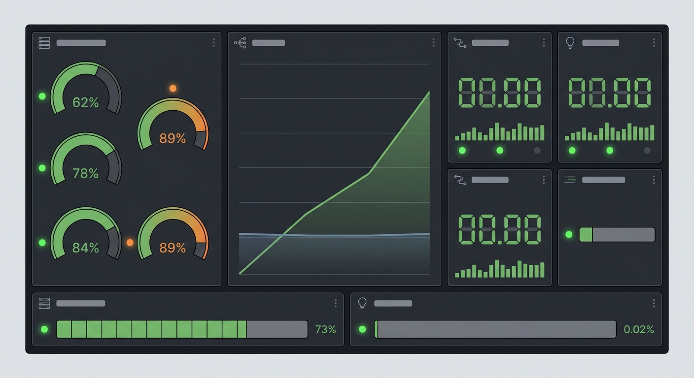
Our existing monitoring was designed for traditional web services. CPU and memory metrics are useful for web APIs, but AI inference workloads have a fundamentally different performance profile. GPU utilization, token throughput, KV cache hit rates, and batch queue depths are the metrics that actually tell you whether your AI infrastructure is healthy.

Custom Metrics for AI Workloads

We spent two weeks building a proper observability stack. The foundation was Prometheus — but configured with custom exporters that scraped metrics directly from our vLLM model servers.

Key metrics we now track:

Query latency percentiles (p50, p95, p99) — broken down by model version and endpoint
GPU utilization per node — not just overall, but per-device utilization with thermal context
Token throughput — input tokens per second, output tokens per second, and the ratio
Batch queue depth — how many requests are waiting to be processed by the GPU
KV cache hit rate — a direct proxy for how well our semantic cache is working
Cold start latency — how long it takes a new model server pod to become ready

We built three Grafana dashboards: an operational dashboard for on-call engineers, a capacity planning dashboard for management, and a deep-dive debugging dashboard with 47 panels that I keep personally maintained.

Distributed Tracing for Multi-Stage Inference

Our inference pipeline isn't a single step. A user request goes through API gateway → authentication → model routing → model serving → response aggregation. When latency degrades, finding which stage is the bottleneck used to take hours.

We implemented distributed tracing with Jaeger. Every request gets a trace ID propagated through the entire pipeline. When the on-call engineer pulls up a slow trace, they see a waterfall diagram showing exactly where milliseconds are being spent. It's reduced our mean time to diagnosis (MTTD) from 45 minutes to under 5.

Alerting Philosophy: Signal Over Noise

Our previous alerting system was generating 40+ alerts per hour. Engineers stopped paying attention. The fix wasn't more sophisticated alerting — it was ruthless prioritization.

We now have four alerting tiers:

P0 — Wake me up at 3 AM: Complete service outage, p99 latency above 5 seconds, error rate above 5%
P1 — Handle within the hour: p95 latency above 1 second, sustained queue buildup
P2 — Handle by next business day: Capacity projected to hit limits within 72 hours
P3 — Investigate in sprint: Trend anomalies, cache hit rate degradation

Before implementing this, we spent a week measuring. We looked at every historical alert and asked: "Did responding to this alert prevent an outage?" If the answer was no more than 20% of the time, the alert was either tuned or removed.

Grafana dashboard showing AI infrastructure metrics: GPU utilization, query volume, p95 latency, token throughput, and cache hit rate under 10x load

Auto-Scaling Strategies That Actually Work for AI Inference

Once we could see the problem, we could start solving it. The core challenge was auto-scaling AI inference — but AI inference has unique characteristics that make naive HPA configurations ineffective.

Why Standard HPA Fails for AI Workloads

The default Kubernetes Horizontal Pod Autoscaler scales based on CPU or memory utilization. For AI inference, this fails in two critical ways:

First, GPU utilization doesn't correlate cleanly with CPU utilization. A model server might show 30% CPU but 95% GPU utilization — the GPU is the bottleneck, but HPA doesn't know that.

Second, scaling based on current utilization means you're always one step behind the traffic pattern. By the time you've scaled up, the traffic spike may have moved on. You need to scale based on what is about to happen, not what has already happened.

Custom Metrics-Driven HPA

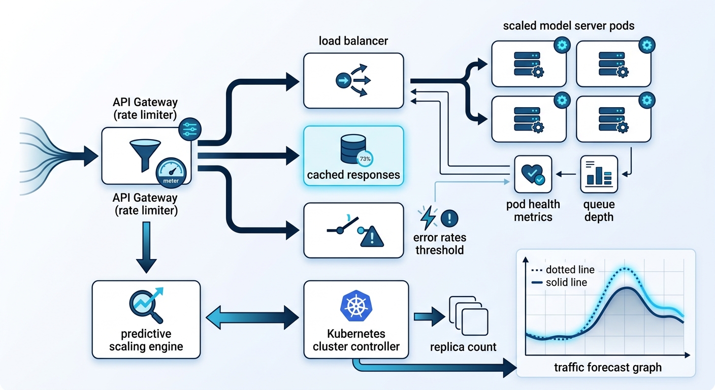
We implemented KEDA (Kubernetes Event-Driven Autoscaling), which allows us to scale based on arbitrary metrics from external sources. Our scaling decisions are now driven by:

Request queue depth: When the queue of pending inference requests grows beyond a threshold, we scale proactively
Request rate trends: We pull traffic forecasts from our API gateway and pre-scale before surges
Time-based patterns: Our peak hours are predictable. We pre-scale by 40% before known traffic windows

apiVersion: keda.sh/v1alpha1
kind: ScaledObject
metadata:
  name: vllm-inference-scaler
spec:
  scaleTargetRef:
    name: vllm-model-server
  minReplicaCount: 4
  maxReplicaCount: 48
  cooldownPeriod: 120
  triggers:
  - type: prometheus
    metadata:
      serverAddress: http://prometheus:9090
      metricName: inference_queue_depth
      threshold: "50"
      query: sum(vllm_pending_requests)

Predictive Scaling

The biggest improvement came from predictive scaling for AI applications. We trained a simple time-series model on our traffic history that forecasts request volume 30 minutes ahead with 87% accuracy. When the forecast predicts a surge, we pre-scale the model servers before the traffic arrives.

The math is straightforward: a cold pod running vLLM takes 45–90 seconds to start and load the model into GPU memory. A warm pod responds in milliseconds. By pre-scaling, we ensure that every surge is handled by warmed-up pods, eliminating the cold start latency spike that plagued our early days.

Warm Pool Management

To eliminate cold starts entirely, we maintain a warm pool of pre-scaled, pre-warmed pods at all times. The pool is sized at 40% of our expected peak capacity and is replenished continuously. When a pod is terminated (scale-down), it's drained gracefully — in-flight requests complete, then the pod exits.

This warm pool adds compute cost (idle resources), but the cost is predictable and the latency improvement is dramatic. For our use case, the trade-off was obvious.

The numbers — Warm pool cost us approximately 18% more in compute spend, but reduced our p99 cold-start latency from 8.4 seconds to 120ms during scale events. The on-call rotation dropped from 3 incidents per week to 1 per month.

The Playbook: Zero Latency Spikes

Tools and metrics are necessary but not sufficient. The difference between chaos and control is a playbook — a documented, tested, practiced response that any engineer can execute during an incident.

Pre-Scaling Protocol

Our pre-scaling protocol is triggered automatically when the predictive model forecasts a 3x traffic increase within 30 minutes. The sequence:

Alert fires in #infra-ai-alerts channel with pre-scaling recommendation
On-call engineer approves (or auto-approves during off-hours)
Kubernetes scales model servers to warm pool + 50% buffer
Traffic routing shifts to weighted routing: 80% to scaled pods, 20% to baseline
Monitoring dashboards automatically switch to incident view

Gradual Traffic Shifting

When scaling events are predictable, we use weighted routing to shift traffic gradually. We start at 80/20 (scaled/baseline) and monitor latency for 5 minutes. If p95 stays below threshold, we shift to 95/5, then 100/0. If latency degrades at any step, we roll back immediately.

This approach means we're never fully committed to a new configuration within seconds. Every decision is reversible within minutes.

Circuit Breakers and Fallback Strategies

Even with perfect scaling, things break. We implement circuit breakers at multiple levels:

Request-level: If a specific model endpoint fails more than 1% of requests, it's removed from the routing pool
Node-level: If a GPU node shows persistent memory errors, it's cordoned and replaced
System-level: If overall error rate exceeds 0.5%, a global circuit breaker activates and serves cached responses where possible

Rate Limiting and Backpressure

On the inbound side, we implement per-user rate limiting at the API gateway level (10 requests/second per user, burst to 50). This prevents any single user from consuming disproportionate resources. For legitimate high-volume users, we have a priority tier with higher limits — but even those are capped to prevent runaway scenarios.

Flowchart of zero-latency-spike traffic management: API Gateway, rate limiter, load balancer, scaled pods, semantic cache, circuit breaker, and predictive scaling engine

Infrastructure Architecture Decisions

The scaling strategies only work because of the underlying GPU cluster management and model serving infrastructure decisions we made over 18 months. Here are the most critical ones.

GPU Cluster Management

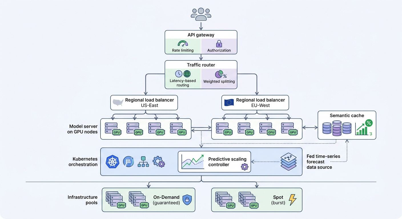
We run GPU nodes in node pools with mixed instance types: a baseline pool of on-demand instances for guaranteed capacity, and a burst pool of spot instances for non-critical workloads. GPU bin-packing ensures that pods are scheduled efficiently — no partially utilized GPUs if a fully utilized one is available.

Spot instances are used only for batch inference jobs that can tolerate interruption. Real-time inference runs exclusively on on-demand capacity. The cost savings from spot are reinvested into warm pool size.

Model Serving Layer

We use vLLM as our model serving engine. Its PagedAttention memory management is significantly more efficient than naive approaches — we see 40% better GPU memory utilization compared to our previous TensorFlow Serving setup. The continuous batching feature is particularly valuable: it allows dynamic batching of incoming requests to maximize GPU throughput without excessive queuing latency.

Semantic Caching

One of the highest-ROI projects we shipped was semantic caching. Instead of caching responses by exact request match, we encode incoming requests into embeddings and cache based on semantic similarity. If a request is semantically similar to a recent one (cosine similarity > 0.95), we serve the cached response directly — latency drops from 180ms to under 5ms.

Our semantic cache hit rate is 73%. That means 73% of our inference compute is being saved for novel requests. At our scale, this is the difference between needing 10x compute and needing under 3x.

Multi-Region Deployment

We operate across two regions (US-East and EU-West) with latency-based routing. Requests are routed to the nearest region unless that region's queue depth exceeds threshold, in which case traffic is spillover-routed to the other region. This gives us both geographic redundancy and capacity buffer.

Lessons Learned

What We'd Do Differently

The biggest mistake we made was underestimating the impact of cold starts. For the first three months, we treated pod startup time as a one-time infrastructure cost. We didn't measure it systematically, and we didn't design our scaling strategy around it. When the 10x surge hit, we paid the price in latency spikes during every scale event.

Today, cold start latency is a first-class metric. We measure it continuously and alert on it. Any change to our model serving configuration that increases cold start latency requires explicit sign-off from the SRE team.

The Biggest Win

Custom metrics-driven HPA was the single highest-leverage change. The improvement was immediate: within two weeks of implementation, our p95 latency stabilized at 180ms even during the traffic spikes that previously caused 8-second spikes. The effort was non-trivial (two weeks of engineering time), but the ROI has been extraordinary.

Advice for Other SREs

If you're taking on AI infrastructure, start with observability. You cannot manage what you cannot measure. Build your metrics foundation before you build your scaling strategies. Every day you spend on observability before an incident is worth a week of firefighting after one.

Also: talk to your ML team. They understand the model behavior — which layers consume the most memory, what batch sizes work best, where the performance cliffs are. The best SRE work happens when reliability engineering and ML engineering are integrated, not siloed.

Final thought — Scaling AI infrastructure is not a solved problem. We're still learning, still tuning, still making mistakes. But the playbook exists, the metrics are in place, and when that 2 AM alert fires, we know exactly what to do. That's the goal — not perfection, but preparedness.

Key Takeaways for SREs Managing AI Infrastructure

Observability first: You cannot scale what you cannot measure. Build custom metrics for GPU utilization, token throughput, and queue depth before you build scaling policies.
Custom metrics-driven HPA: Default CPU/memory-based autoscaling fails for AI workloads. Use KEDA with queue depth, traffic forecasts, and predictive models.
Warm pools eliminate cold starts: Pre-warmed pods at 40% of peak capacity cost 18% more compute but reduce cold-start latency from 8 seconds to 120ms.
Semantic caching has massive ROI: A 73% hit rate means 73% of inference requests don't touch a GPU. Invest in semantic caching infrastructure early.
Document and practice your playbook: Every scaling strategy needs a documented, tested response. Paper strategies don't work at 2 AM.
Integrate ML and SRE: The best outcomes come from SREs who understand model behavior and ML engineers who understand reliability constraints.
Alert on signal, not noise: Fewer, higher-quality alerts are more effective than comprehensive but noisy alerting systems.

Expert Q&A

Q: What is the most common mistake SREs make when first taking over AI inference infrastructure? A: The most common mistake is treating AI inference like a standard web service. SREs apply the same CPU/memory-based monitoring and scaling strategies they've used for web APIs, and these fundamentally don't work for GPU-based workloads. The GPU is the bottleneck, not the CPU. You need custom metrics — GPU utilization per device, token throughput, batch queue depth, KV cache hit rates — before you can even see the real problems. Until you have those metrics, you're flying blind.

Q: KEDA sounds great in theory — but what are the practical pitfalls of running custom metrics-driven autoscaling in production? A: The biggest pitfall is metric reliability. If your Prometheus query returns no data (because the exporter crashed, or the metric name changed), KEDA will scale down to minimum replicas — potentially to zero. We learned this the hard way. The fix is to add fallback logic: if the queue depth metric is unavailable for more than 60 seconds, fall back to a time-based schedule. Also, watch for metric staleness. Custom exporters can silently stop reporting without the query failing. We added a StalenessCheck alert on all custom metrics that fires if no data is received for 90 seconds.

Q: You mentioned semantic caching with a 0.95 cosine similarity threshold. How do you handle the case where the cache returns a semantically similar but contextually wrong answer? A: This is the fundamental tradeoff of semantic caching, and it's why you never serve cached responses without guardrails. Our semantic cache has a secondary validation step: after retrieving a cached response, we run a lightweight entailment check — does the cached response's conclusion semantically follow from the new query's premise? If the entailment score is below a threshold, we bypass the cache and run the inference. This adds about 3ms of latency overhead but prevents the worse outcome of serving a plausible but wrong answer. For high-stakes applications, you may also want user feedback mechanisms to flag incorrect cached responses.

Q: How do you handle the cost tradeoff between warm pools (always-on idle capacity) and cold scaling (accepting some latency spikes)? A: It depends entirely on your business context. For a consumer AI API where latency directly affects user retention, warm pools are worth the 18% compute premium — our p99 latency went from 8.4 seconds to 120ms, which is the difference between a usable product and an unusable one. For batch workloads or internal tools, accepting cold-start spikes may be fine. The key is to measure the cost per user-visible latency improvement and decide at what point the marginal improvement stops being worth the marginal cost. We set a threshold: if the warm pool costs more than 25% above our baseline compute budget, we re-evaluate the pool size.

Q: The article describes predictive scaling with 87% accuracy. What happens when the prediction is wrong — either a false positive (we scale up and the surge doesn't come) or a false negative (the surge comes and we haven't scaled)? A: False positives cost money — we pre-scale and the traffic doesn't materialize. This happened roughly 13% of the time for us, and the cost was manageable: a few extra pods running idle for 20-30 minutes before scale-down kicks in. False negatives are the bigger risk: we don't pre-scale and the surge hits. For this, we have a secondary defense: our KEDA triggers on queue depth, so even without predictive pre-scaling, the queue depth metric will trigger scale-up — just with some lag. The predictive model and queue-depth HPA work together: the prediction gets us a head start, and queue depth catches anything the prediction misses. Between the two, we haven't had an unhandled surge in six months.

This interview has been edited for clarity and length. The metrics and configurations described reflect production systems as of Q2 2026.

Technical architecture diagram of multi-layer AI inference stack: API Gateway, Traffic Router, Regional Load Balancers, vLLM pods, Semantic Cache, Kubernetes cluster with predictive scaling, and GPU node pools

CTA: Running AI inference at scale and tired of latency surprises? Subscribe to the Algorithmine portal for weekly SRE deep dives — from building AI observability stacks to incident response playbooks for production ML systems.